Transcriptomics following RNAi
Devon Boland and Maeva Techer
2026-04-06
Last updated: 2026-04-06
Checks: 6 1
Knit directory:
locust-comparative-genomics/
This reproducible R Markdown analysis was created with workflowr (version 1.7.2). The Checks tab describes the reproducibility checks that were applied when the results were created. The Past versions tab lists the development history.
Great! Since the R Markdown file has been committed to the Git repository, you know the exact version of the code that produced these results.
Great job! The global environment was empty. Objects defined in the global environment can affect the analysis in your R Markdown file in unknown ways. For reproduciblity it’s best to always run the code in an empty environment.
The command set.seed(20221025) was run prior to running
the code in the R Markdown file. Setting a seed ensures that any results
that rely on randomness, e.g. subsampling or permutations, are
reproducible.
Great job! Recording the operating system, R version, and package versions is critical for reproducibility.
Nice! There were no cached chunks for this analysis, so you can be confident that you successfully produced the results during this run.
Using absolute paths to the files within your workflowr project makes it difficult for you and others to run your code on a different machine. Change the absolute path(s) below to the suggested relative path(s) to make your code more reproducible.
| absolute | relative |
|---|---|
| /Users/maevatecher/Documents/GitHub/locust-comparative-genomics/data/RefSeq/GCF_023897955.1_iqSchGreg1.2_genomic.gtf | data/RefSeq/GCF_023897955.1_iqSchGreg1.2_genomic.gtf |
| /Users/maevatecher/Documents/GitHub/locust-comparative-genomics/data/list/GO_Annotations/blast2go_gregaria.annot.mgp_removed | data/list/GO_Annotations/blast2go_gregaria.annot.mgp_removed |
| /Users/maevatecher/Documents/GitHub/locust-comparative-genomics/data/custom_sgregaria_orgdb | data/custom_sgregaria_orgdb |
| /Users/maevatecher/Documents/GitHub/locust-comparative-genomics/data/custom_sgregaria_orgdb/org.Sgregaria.eg.db | data/custom_sgregaria_orgdb/org.Sgregaria.eg.db |
| /Users/maevatecher/Documents/GitHub/locust-comparative-genomics/data | data |
Great! You are using Git for version control. Tracking code development and connecting the code version to the results is critical for reproducibility.
The results in this page were generated with repository version 3f5c874. See the Past versions tab to see a history of the changes made to the R Markdown and HTML files.
Note that you need to be careful to ensure that all relevant files for
the analysis have been committed to Git prior to generating the results
(you can use wflow_publish or
wflow_git_commit). workflowr only checks the R Markdown
file, but you know if there are other scripts or data files that it
depends on. Below is the status of the Git repository when the results
were generated:
Ignored files:
Ignored: .DS_Store
Ignored: .Rhistory
Ignored: analysis/.DS_Store
Ignored: analysis/.Rhistory
Ignored: analysis/2_signatures-selection_cache/
Ignored: analysis/3_wgcna-network_cache/
Ignored: analysis/figure/
Ignored: code/.DS_Store
Ignored: code/scripts/.DS_Store
Ignored: code/scripts/pal2nal.v14/.DS_Store
Ignored: data/.DS_Store
Ignored: data/DEG_results/.DS_Store
Ignored: data/DEG_results/Bulk_RNAseq/.DS_Store
Ignored: data/DEG_results/Bulk_RNAseq/americana/.DS_Store
Ignored: data/DEG_results/Bulk_RNAseq/cancellata/.DS_Store
Ignored: data/DEG_results/Bulk_RNAseq/cubense/.DS_Store
Ignored: data/DEG_results/Bulk_RNAseq/gregaria/.DS_Store
Ignored: data/DEG_results/Bulk_RNAseq/nitens/.DS_Store
Ignored: data/DEG_results/RNAi/.DS_Store
Ignored: data/DEG_results/RNAi/All_control_no_rRNA/.DS_Store
Ignored: data/DEG_results/RNAi/Head/.DS_Store
Ignored: data/DEG_results/RNAi/Head_control/.DS_Store
Ignored: data/DEG_results/RNAi/Head_no_rRNA/.DS_Store
Ignored: data/DEG_results/RNAi/Thorax/.DS_Store
Ignored: data/HYPHY_selection/.DS_Store
Ignored: data/HYPHY_selection/ParsedABSRELResults_unlabeled/.DS_Store
Ignored: data/HYPHY_selection/functional_pathways/.DS_Store
Ignored: data/HYPHY_selection/functional_pathways/aBSREL/.DS_Store
Ignored: data/HYPHY_selection/pathway_enrichment/.DS_Store
Ignored: data/HYPHY_selection/pathway_enrichment/americana/
Ignored: data/HYPHY_selection/pathway_enrichment/cancellata/
Ignored: data/HYPHY_selection/pathway_enrichment/cubense/
Ignored: data/HYPHY_selection/pathway_enrichment/nitens/
Ignored: data/HYPHY_selection/pathway_enrichment/piceifrons/
Ignored: data/WGCNA/.DS_Store
Ignored: data/WGCNA/input/.DS_Store
Ignored: data/WGCNA/input/Bulk_RNAseq/.DS_Store
Ignored: data/WGCNA/input/GRNs/.DS_Store
Ignored: data/WGCNA/output/.DS_Store
Ignored: data/WGCNA/output/Bulk_RNAseq/.DS_Store
Ignored: data/WGCNA/output/Bulk_RNAseq/americana/
Ignored: data/WGCNA/output/Bulk_RNAseq/gregaria/.DS_Store
Ignored: data/WGCNA/output/Bulk_RNAseq/gregaria/Head/
Ignored: data/WGCNA/output/Bulk_RNAseq/gregaria/Thorax/
Ignored: data/behavioral_data/.DS_Store
Ignored: data/behavioral_data/Raw_data/.DS_Store
Ignored: data/cafe5_results/.DS_Store
Ignored: data/cafe5_results/Base_change_FILE/.DS_Store
Ignored: data/cafe5_results/Base_change_FILE/americana/.DS_Store
Ignored: data/cafe5_results/Base_change_FILE/gregaria/.DS_Store
Ignored: data/cafe5_results/Base_change_FILE/locusta/.DS_Store
Ignored: data/cafe5_results/Gene_count_FILE/.DS_Store
Ignored: data/list/.DS_Store
Ignored: data/list/Bulk_RNAseq/.DS_Store
Ignored: data/list/GO_Annotations/.DS_Store
Ignored: data/list/GO_Annotations/DesertLocustR/.DS_Store
Ignored: data/list/excluded_loci/.DS_Store
Ignored: data/orthofinder/.DS_Store
Ignored: data/orthofinder/Polyneoptera/.DS_Store
Ignored: data/orthofinder/Polyneoptera/Results_I2_iqtree/.DS_Store
Ignored: data/orthofinder/Polyneoptera/Results_I2_iqtree/Orthogroups/.DS_Store
Ignored: data/orthofinder/Polyneoptera/Results_I2_withDaust/.DS_Store
Ignored: data/orthofinder/Polyneoptera/Results_I2_withDaust/Orthogroups/.DS_Store
Ignored: data/orthofinder/Schistocerca/.DS_Store
Ignored: data/orthofinder/Schistocerca/Results_I2/.DS_Store
Ignored: data/orthofinder/Schistocerca/Results_I2/Orthogroups/.DS_Store
Ignored: data/overlap/.DS_Store
Ignored: data/pathway_enrichment/.DS_Store
Ignored: data/pathway_enrichment/OLD/.DS_Store
Ignored: data/pathway_enrichment/OLD/custom_sgregaria_orgdb/.DS_Store
Ignored: data/pathway_enrichment/REVIGO_results/.DS_Store
Ignored: data/pathway_enrichment/REVIGO_results/BP/.DS_Store
Ignored: data/pathway_enrichment/REVIGO_results/CC/.DS_Store
Ignored: data/pathway_enrichment/REVIGO_results/MF/.DS_Store
Ignored: data/pathway_enrichment/americana/.DS_Store
Ignored: data/pathway_enrichment/cancellata/.DS_Store
Ignored: data/pathway_enrichment/gregaria/.DS_Store
Ignored: data/pathway_enrichment/nitens/Thorax/
Ignored: data/pathway_enrichment/piceifrons/.DS_Store
Ignored: data/readcounts/.DS_Store
Ignored: data/readcounts/Bulk_RNAseq/.DS_Store
Ignored: data/readcounts/RNAi/.DS_Store
Untracked files:
Untracked: VennDiagram.2026-04-06_23-47-16.411955.log
Untracked: VennDiagram.2026-04-06_23-47-17.210952.log
Untracked: VennDiagram.2026-04-06_23-47-17.665755.log
Untracked: VennDiagram.2026-04-06_23-47-18.161976.log
Untracked: VennDiagram.2026-04-06_23-47-18.653184.log
Untracked: VennDiagram.2026-04-06_23-47-19.194583.log
Untracked: VennDiagram.2026-04-06_23-47-19.268816.log
Untracked: VennDiagram.2026-04-06_23-47-19.399468.log
Untracked: VennDiagram.2026-04-06_23-47-20.051671.log
Untracked: VennDiagram.2026-04-06_23-47-20.11203.log
Untracked: VennDiagram.2026-04-06_23-47-20.227166.log
Untracked: VennDiagram.2026-04-06_23-47-21.166017.log
Untracked: VennDiagram.2026-04-06_23-47-21.203171.log
Untracked: VennDiagram.2026-04-06_23-47-21.312708.log
Untracked: VennDiagram.2026-04-06_23-47-21.830603.log
Untracked: VennDiagram.2026-04-06_23-47-21.865964.log
Untracked: VennDiagram.2026-04-06_23-47-21.92949.log
Untracked: VennDiagram.2026-04-06_23-47-22.550008.log
Untracked: VennDiagram.2026-04-06_23-47-22.64388.log
Untracked: VennDiagram.2026-04-06_23-47-22.791879.log
Untracked: VennDiagram.2026-04-06_23-47-23.475483.log
Untracked: VennDiagram.2026-04-06_23-47-23.614065.log
Untracked: VennDiagram.2026-04-06_23-47-23.715451.log
Untracked: VennDiagram.2026-04-06_23-47-24.707496.log
Untracked: VennDiagram.2026-04-06_23-47-24.828032.log
Untracked: VennDiagram.2026-04-06_23-47-24.961809.log
Untracked: VennDiagram.2026-04-06_23-47-25.081758.log
Untracked: VennDiagram.2026-04-06_23-47-25.213998.log
Untracked: VennDiagram.2026-04-06_23-47-25.346891.log
Untracked: analysis/bustedPH_logomega3_scatter_nosuspect.pdf
Untracked: bustedPH_logomega3_scatter_nosuspect.pdf
Untracked: data/HYPHY_selection/functional_pathways/BUSTED_unlabeled/
Untracked: data/RefSeq/
Untracked: data/WGCNA/output/Bulk_RNAseq/cancellata/
Untracked: data/WGCNA/output/Bulk_RNAseq/gregaria/ModuleTraitRelationships_Head_gregaria_with_colors_name_filter.pdf
Untracked: data/WGCNA/output/Bulk_RNAseq/piceifrons/
Untracked: data/orthofinder/Polyneoptera/Results_I2_iqtree/trusted_ogs_v2.txt
Unstaged changes:
Deleted: analysis/2_hic-snps-phylogeny.Rmd
Modified: analysis/3_wgcna-network.Rmd
Modified: analysis/4_RNAi_behavior.Rmd
Modified: analysis/_site.yml
Modified: data/DEG_results/Bulk_RNAseq/americana/Head/MA_plot_DEG_Head_igris.png
Modified: data/DEG_results/Bulk_RNAseq/americana/Head/MA_plot_DEG_Head_igris_togregaria.png
Modified: data/DEG_results/Bulk_RNAseq/americana/Head/heatmap_VST_Head.pdf
Modified: data/DEG_results/Bulk_RNAseq/americana/Head/heatmap_VST_Head_togregaria.pdf
Modified: data/DEG_results/Bulk_RNAseq/americana/Head/heatmap_normTransform_Head.pdf
Modified: data/DEG_results/Bulk_RNAseq/americana/Head/heatmap_normTransform_Head_togregaria.pdf
Modified: data/DEG_results/Bulk_RNAseq/americana/Head/heatmap_rlog_Head.pdf
Modified: data/DEG_results/Bulk_RNAseq/americana/Head/heatmap_rlog_Head_togregaria.pdf
Modified: data/DEG_results/Bulk_RNAseq/americana/Head/sva_scatter_SV1_SV2_Head.png
Modified: data/DEG_results/Bulk_RNAseq/americana/Head/sva_scatter_SV1_SV2_Head_togregaria.png
Modified: data/DEG_results/Bulk_RNAseq/americana/Head/sva_scatter_SV1_SV3_Head.png
Modified: data/DEG_results/Bulk_RNAseq/americana/Head/sva_scatter_SV1_SV3_Head_togregaria.png
Modified: data/DEG_results/Bulk_RNAseq/americana/Head/sva_scatter_SV2_SV3_Head.png
Modified: data/DEG_results/Bulk_RNAseq/americana/Head/sva_scatter_SV2_SV3_Head_togregaria.png
Modified: data/DEG_results/Bulk_RNAseq/americana/Head/sva_stripchart_SV1_Head.png
Modified: data/DEG_results/Bulk_RNAseq/americana/Head/sva_stripchart_SV1_Head_togregaria.png
Modified: data/DEG_results/Bulk_RNAseq/americana/Head/sva_stripchart_SV2_Head.png
Modified: data/DEG_results/Bulk_RNAseq/americana/Head/sva_stripchart_SV2_Head_togregaria.png
Modified: data/DEG_results/Bulk_RNAseq/americana/Head/sva_stripchart_SV3_Head.png
Modified: data/DEG_results/Bulk_RNAseq/americana/Head/sva_stripchart_SV3_Head_togregaria.png
Modified: data/DEG_results/Bulk_RNAseq/americana/Head/volcano_DEG_Head_igris.png
Modified: data/DEG_results/Bulk_RNAseq/americana/Head/volcano_DEG_Head_igris_togregaria.png
Modified: data/DEG_results/Bulk_RNAseq/americana/Thorax/MA_plot_DEG_Thorax_igris.png
Modified: data/DEG_results/Bulk_RNAseq/americana/Thorax/MA_plot_DEG_Thorax_igris_togregaria.png
Modified: data/DEG_results/Bulk_RNAseq/americana/Thorax/heatmap_VST_Thorax.pdf
Modified: data/DEG_results/Bulk_RNAseq/americana/Thorax/heatmap_VST_Thorax_togregaria.pdf
Modified: data/DEG_results/Bulk_RNAseq/americana/Thorax/heatmap_normTransform_Thorax.pdf
Modified: data/DEG_results/Bulk_RNAseq/americana/Thorax/heatmap_normTransform_Thorax_togregaria.pdf
Modified: data/DEG_results/Bulk_RNAseq/americana/Thorax/heatmap_rlog_Thorax.pdf
Modified: data/DEG_results/Bulk_RNAseq/americana/Thorax/heatmap_rlog_Thorax_togregaria.pdf
Modified: data/DEG_results/Bulk_RNAseq/americana/Thorax/sva_scatter_SV1_SV2_Thorax.png
Modified: data/DEG_results/Bulk_RNAseq/americana/Thorax/sva_scatter_SV1_SV2_Thorax_togregaria.png
Modified: data/DEG_results/Bulk_RNAseq/americana/Thorax/sva_scatter_SV1_SV3_Thorax.png
Modified: data/DEG_results/Bulk_RNAseq/americana/Thorax/sva_scatter_SV1_SV3_Thorax_togregaria.png
Modified: data/DEG_results/Bulk_RNAseq/americana/Thorax/sva_scatter_SV2_SV3_Thorax.png
Modified: data/DEG_results/Bulk_RNAseq/americana/Thorax/sva_scatter_SV2_SV3_Thorax_togregaria.png
Modified: data/DEG_results/Bulk_RNAseq/americana/Thorax/sva_stripchart_SV1_Thorax.png
Modified: data/DEG_results/Bulk_RNAseq/americana/Thorax/sva_stripchart_SV1_Thorax_togregaria.png
Modified: data/DEG_results/Bulk_RNAseq/americana/Thorax/sva_stripchart_SV2_Thorax.png
Modified: data/DEG_results/Bulk_RNAseq/americana/Thorax/sva_stripchart_SV2_Thorax_togregaria.png
Modified: data/DEG_results/Bulk_RNAseq/americana/Thorax/sva_stripchart_SV3_Thorax.png
Modified: data/DEG_results/Bulk_RNAseq/americana/Thorax/sva_stripchart_SV3_Thorax_togregaria.png
Modified: data/DEG_results/Bulk_RNAseq/americana/Thorax/volcano_DEG_Thorax_igris.png
Modified: data/DEG_results/Bulk_RNAseq/americana/Thorax/volcano_DEG_Thorax_igris_togregaria.png
Modified: data/DEG_results/Bulk_RNAseq/cancellata/Head/MA_plot_DEG_Head_igris.png
Modified: data/DEG_results/Bulk_RNAseq/cancellata/Head/MA_plot_DEG_Head_igris_togregaria.png
Modified: data/DEG_results/Bulk_RNAseq/cancellata/Head/heatmap_VST_Head.pdf
Modified: data/DEG_results/Bulk_RNAseq/cancellata/Head/heatmap_VST_Head_togregaria.pdf
Modified: data/DEG_results/Bulk_RNAseq/cancellata/Head/heatmap_normTransform_Head.pdf
Modified: data/DEG_results/Bulk_RNAseq/cancellata/Head/heatmap_normTransform_Head_togregaria.pdf
Modified: data/DEG_results/Bulk_RNAseq/cancellata/Head/heatmap_rlog_Head.pdf
Modified: data/DEG_results/Bulk_RNAseq/cancellata/Head/heatmap_rlog_Head_togregaria.pdf
Modified: data/DEG_results/Bulk_RNAseq/cancellata/Head/sva_scatter_SV1_SV2_Head.png
Modified: data/DEG_results/Bulk_RNAseq/cancellata/Head/sva_scatter_SV1_SV2_Head_togregaria.png
Modified: data/DEG_results/Bulk_RNAseq/cancellata/Head/sva_scatter_SV1_SV3_Head.png
Modified: data/DEG_results/Bulk_RNAseq/cancellata/Head/sva_scatter_SV1_SV3_Head_togregaria.png
Modified: data/DEG_results/Bulk_RNAseq/cancellata/Head/sva_scatter_SV2_SV3_Head.png
Modified: data/DEG_results/Bulk_RNAseq/cancellata/Head/sva_scatter_SV2_SV3_Head_togregaria.png
Modified: data/DEG_results/Bulk_RNAseq/cancellata/Head/sva_stripchart_SV1_Head.png
Modified: data/DEG_results/Bulk_RNAseq/cancellata/Head/sva_stripchart_SV1_Head_togregaria.png
Modified: data/DEG_results/Bulk_RNAseq/cancellata/Head/sva_stripchart_SV2_Head.png
Modified: data/DEG_results/Bulk_RNAseq/cancellata/Head/sva_stripchart_SV2_Head_togregaria.png
Modified: data/DEG_results/Bulk_RNAseq/cancellata/Head/sva_stripchart_SV3_Head.png
Modified: data/DEG_results/Bulk_RNAseq/cancellata/Head/sva_stripchart_SV3_Head_togregaria.png
Modified: data/DEG_results/Bulk_RNAseq/cancellata/Head/volcano_DEG_Head_igris.png
Modified: data/DEG_results/Bulk_RNAseq/cancellata/Head/volcano_DEG_Head_igris_togregaria.png
Modified: data/DEG_results/Bulk_RNAseq/cancellata/Thorax/MA_plot_DEG_Thorax_igris.png
Modified: data/DEG_results/Bulk_RNAseq/cancellata/Thorax/MA_plot_DEG_Thorax_igris_togregaria.png
Modified: data/DEG_results/Bulk_RNAseq/cancellata/Thorax/heatmap_VST_Thorax.pdf
Modified: data/DEG_results/Bulk_RNAseq/cancellata/Thorax/heatmap_VST_Thorax_togregaria.pdf
Modified: data/DEG_results/Bulk_RNAseq/cancellata/Thorax/heatmap_normTransform_Thorax.pdf
Modified: data/DEG_results/Bulk_RNAseq/cancellata/Thorax/heatmap_normTransform_Thorax_togregaria.pdf
Modified: data/DEG_results/Bulk_RNAseq/cancellata/Thorax/heatmap_rlog_Thorax.pdf
Modified: data/DEG_results/Bulk_RNAseq/cancellata/Thorax/heatmap_rlog_Thorax_togregaria.pdf
Modified: data/DEG_results/Bulk_RNAseq/cancellata/Thorax/sva_scatter_SV1_SV2_Thorax.png
Modified: data/DEG_results/Bulk_RNAseq/cancellata/Thorax/sva_scatter_SV1_SV2_Thorax_togregaria.png
Modified: data/DEG_results/Bulk_RNAseq/cancellata/Thorax/sva_scatter_SV1_SV3_Thorax.png
Modified: data/DEG_results/Bulk_RNAseq/cancellata/Thorax/sva_scatter_SV1_SV3_Thorax_togregaria.png
Modified: data/DEG_results/Bulk_RNAseq/cancellata/Thorax/sva_scatter_SV2_SV3_Thorax.png
Modified: data/DEG_results/Bulk_RNAseq/cancellata/Thorax/sva_scatter_SV2_SV3_Thorax_togregaria.png
Modified: data/DEG_results/Bulk_RNAseq/cancellata/Thorax/sva_stripchart_SV1_Thorax.png
Modified: data/DEG_results/Bulk_RNAseq/cancellata/Thorax/sva_stripchart_SV1_Thorax_togregaria.png
Modified: data/DEG_results/Bulk_RNAseq/cancellata/Thorax/sva_stripchart_SV2_Thorax.png
Modified: data/DEG_results/Bulk_RNAseq/cancellata/Thorax/sva_stripchart_SV2_Thorax_togregaria.png
Modified: data/DEG_results/Bulk_RNAseq/cancellata/Thorax/sva_stripchart_SV3_Thorax.png
Modified: data/DEG_results/Bulk_RNAseq/cancellata/Thorax/sva_stripchart_SV3_Thorax_togregaria.png
Modified: data/DEG_results/Bulk_RNAseq/cancellata/Thorax/volcano_DEG_Thorax_igris.png
Modified: data/DEG_results/Bulk_RNAseq/cancellata/Thorax/volcano_DEG_Thorax_igris_togregaria.png
Modified: data/DEG_results/Bulk_RNAseq/cubense/Head/MA_plot_DEG_Head_igris.png
Modified: data/DEG_results/Bulk_RNAseq/cubense/Head/MA_plot_DEG_Head_igris_togregaria.png
Modified: data/DEG_results/Bulk_RNAseq/cubense/Head/heatmap_VST_Head.pdf
Modified: data/DEG_results/Bulk_RNAseq/cubense/Head/heatmap_VST_Head_togregaria.pdf
Modified: data/DEG_results/Bulk_RNAseq/cubense/Head/heatmap_normTransform_Head.pdf
Modified: data/DEG_results/Bulk_RNAseq/cubense/Head/heatmap_normTransform_Head_togregaria.pdf
Modified: data/DEG_results/Bulk_RNAseq/cubense/Head/heatmap_rlog_Head.pdf
Modified: data/DEG_results/Bulk_RNAseq/cubense/Head/heatmap_rlog_Head_togregaria.pdf
Modified: data/DEG_results/Bulk_RNAseq/cubense/Head/sva_scatter_SV1_SV2_Head.png
Modified: data/DEG_results/Bulk_RNAseq/cubense/Head/sva_scatter_SV1_SV2_Head_togregaria.png
Modified: data/DEG_results/Bulk_RNAseq/cubense/Head/sva_scatter_SV1_SV3_Head.png
Modified: data/DEG_results/Bulk_RNAseq/cubense/Head/sva_scatter_SV1_SV3_Head_togregaria.png
Modified: data/DEG_results/Bulk_RNAseq/cubense/Head/sva_scatter_SV2_SV3_Head.png
Modified: data/DEG_results/Bulk_RNAseq/cubense/Head/sva_scatter_SV2_SV3_Head_togregaria.png
Modified: data/DEG_results/Bulk_RNAseq/cubense/Head/sva_stripchart_SV1_Head.png
Modified: data/DEG_results/Bulk_RNAseq/cubense/Head/sva_stripchart_SV1_Head_togregaria.png
Modified: data/DEG_results/Bulk_RNAseq/cubense/Head/sva_stripchart_SV2_Head.png
Modified: data/DEG_results/Bulk_RNAseq/cubense/Head/sva_stripchart_SV2_Head_togregaria.png
Modified: data/DEG_results/Bulk_RNAseq/cubense/Head/sva_stripchart_SV3_Head.png
Modified: data/DEG_results/Bulk_RNAseq/cubense/Head/sva_stripchart_SV3_Head_togregaria.png
Modified: data/DEG_results/Bulk_RNAseq/cubense/Head/volcano_DEG_Head_igris.png
Modified: data/DEG_results/Bulk_RNAseq/cubense/Head/volcano_DEG_Head_igris_togregaria.png
Modified: data/DEG_results/Bulk_RNAseq/cubense/Thorax/MA_plot_DEG_Thorax_igris.png
Modified: data/DEG_results/Bulk_RNAseq/cubense/Thorax/MA_plot_DEG_Thorax_igris_togregaria.png
Modified: data/DEG_results/Bulk_RNAseq/cubense/Thorax/heatmap_VST_Thorax.pdf
Modified: data/DEG_results/Bulk_RNAseq/cubense/Thorax/heatmap_VST_Thorax_togregaria.pdf
Modified: data/DEG_results/Bulk_RNAseq/cubense/Thorax/heatmap_normTransform_Thorax.pdf
Modified: data/DEG_results/Bulk_RNAseq/cubense/Thorax/heatmap_normTransform_Thorax_togregaria.pdf
Modified: data/DEG_results/Bulk_RNAseq/cubense/Thorax/heatmap_rlog_Thorax.pdf
Modified: data/DEG_results/Bulk_RNAseq/cubense/Thorax/heatmap_rlog_Thorax_togregaria.pdf
Modified: data/DEG_results/Bulk_RNAseq/cubense/Thorax/sva_scatter_SV1_SV2_Thorax.png
Modified: data/DEG_results/Bulk_RNAseq/cubense/Thorax/sva_scatter_SV1_SV2_Thorax_togregaria.png
Modified: data/DEG_results/Bulk_RNAseq/cubense/Thorax/sva_scatter_SV1_SV3_Thorax.png
Modified: data/DEG_results/Bulk_RNAseq/cubense/Thorax/sva_scatter_SV1_SV3_Thorax_togregaria.png
Modified: data/DEG_results/Bulk_RNAseq/cubense/Thorax/sva_scatter_SV2_SV3_Thorax.png
Modified: data/DEG_results/Bulk_RNAseq/cubense/Thorax/sva_scatter_SV2_SV3_Thorax_togregaria.png
Modified: data/DEG_results/Bulk_RNAseq/cubense/Thorax/sva_stripchart_SV1_Thorax.png
Modified: data/DEG_results/Bulk_RNAseq/cubense/Thorax/sva_stripchart_SV1_Thorax_togregaria.png
Modified: data/DEG_results/Bulk_RNAseq/cubense/Thorax/sva_stripchart_SV2_Thorax.png
Modified: data/DEG_results/Bulk_RNAseq/cubense/Thorax/sva_stripchart_SV2_Thorax_togregaria.png
Modified: data/DEG_results/Bulk_RNAseq/cubense/Thorax/sva_stripchart_SV3_Thorax.png
Modified: data/DEG_results/Bulk_RNAseq/cubense/Thorax/sva_stripchart_SV3_Thorax_togregaria.png
Modified: data/DEG_results/Bulk_RNAseq/cubense/Thorax/volcano_DEG_Thorax_igris.png
Modified: data/DEG_results/Bulk_RNAseq/cubense/Thorax/volcano_DEG_Thorax_igris_togregaria.png
Modified: data/DEG_results/Bulk_RNAseq/gregaria/Head/MA_plot_DEG_Head_igris.png
Modified: data/DEG_results/Bulk_RNAseq/gregaria/Head/MA_plot_DEG_Head_igris_togregaria.png
Modified: data/DEG_results/Bulk_RNAseq/gregaria/Head/heatmap_VST_Head.pdf
Modified: data/DEG_results/Bulk_RNAseq/gregaria/Head/heatmap_VST_Head_togregaria.pdf
Modified: data/DEG_results/Bulk_RNAseq/gregaria/Head/heatmap_normTransform_Head.pdf
Modified: data/DEG_results/Bulk_RNAseq/gregaria/Head/heatmap_normTransform_Head_togregaria.pdf
Modified: data/DEG_results/Bulk_RNAseq/gregaria/Head/heatmap_rlog_Head.pdf
Modified: data/DEG_results/Bulk_RNAseq/gregaria/Head/heatmap_rlog_Head_togregaria.pdf
Modified: data/DEG_results/Bulk_RNAseq/gregaria/Head/sva_scatter_SV1_SV2_Head.png
Modified: data/DEG_results/Bulk_RNAseq/gregaria/Head/sva_scatter_SV1_SV2_Head_togregaria.png
Modified: data/DEG_results/Bulk_RNAseq/gregaria/Head/sva_scatter_SV1_SV3_Head.png
Modified: data/DEG_results/Bulk_RNAseq/gregaria/Head/sva_scatter_SV1_SV3_Head_togregaria.png
Modified: data/DEG_results/Bulk_RNAseq/gregaria/Head/sva_scatter_SV2_SV3_Head.png
Modified: data/DEG_results/Bulk_RNAseq/gregaria/Head/sva_scatter_SV2_SV3_Head_togregaria.png
Modified: data/DEG_results/Bulk_RNAseq/gregaria/Head/sva_stripchart_SV1_Head.png
Modified: data/DEG_results/Bulk_RNAseq/gregaria/Head/sva_stripchart_SV1_Head_togregaria.png
Modified: data/DEG_results/Bulk_RNAseq/gregaria/Head/sva_stripchart_SV2_Head.png
Modified: data/DEG_results/Bulk_RNAseq/gregaria/Head/sva_stripchart_SV2_Head_togregaria.png
Modified: data/DEG_results/Bulk_RNAseq/gregaria/Head/sva_stripchart_SV3_Head.png
Modified: data/DEG_results/Bulk_RNAseq/gregaria/Head/sva_stripchart_SV3_Head_togregaria.png
Modified: data/DEG_results/Bulk_RNAseq/gregaria/Head/volcano_DEG_Head_igris.png
Modified: data/DEG_results/Bulk_RNAseq/gregaria/Head/volcano_DEG_Head_igris_togregaria.png
Modified: data/DEG_results/Bulk_RNAseq/gregaria/Thorax/MA_plot_DEG_Thorax_igris.png
Modified: data/DEG_results/Bulk_RNAseq/gregaria/Thorax/MA_plot_DEG_Thorax_igris_togregaria.png
Modified: data/DEG_results/Bulk_RNAseq/gregaria/Thorax/heatmap_VST_Thorax.pdf
Modified: data/DEG_results/Bulk_RNAseq/gregaria/Thorax/heatmap_VST_Thorax_togregaria.pdf
Modified: data/DEG_results/Bulk_RNAseq/gregaria/Thorax/heatmap_normTransform_Thorax.pdf
Modified: data/DEG_results/Bulk_RNAseq/gregaria/Thorax/heatmap_normTransform_Thorax_togregaria.pdf
Modified: data/DEG_results/Bulk_RNAseq/gregaria/Thorax/heatmap_rlog_Thorax.pdf
Modified: data/DEG_results/Bulk_RNAseq/gregaria/Thorax/heatmap_rlog_Thorax_togregaria.pdf
Modified: data/DEG_results/Bulk_RNAseq/gregaria/Thorax/sva_scatter_SV1_SV2_Thorax.png
Modified: data/DEG_results/Bulk_RNAseq/gregaria/Thorax/sva_scatter_SV1_SV2_Thorax_togregaria.png
Modified: data/DEG_results/Bulk_RNAseq/gregaria/Thorax/sva_scatter_SV1_SV3_Thorax.png
Modified: data/DEG_results/Bulk_RNAseq/gregaria/Thorax/sva_scatter_SV1_SV3_Thorax_togregaria.png
Modified: data/DEG_results/Bulk_RNAseq/gregaria/Thorax/sva_scatter_SV2_SV3_Thorax.png
Modified: data/DEG_results/Bulk_RNAseq/gregaria/Thorax/sva_scatter_SV2_SV3_Thorax_togregaria.png
Modified: data/DEG_results/Bulk_RNAseq/gregaria/Thorax/sva_stripchart_SV1_Thorax.png
Modified: data/DEG_results/Bulk_RNAseq/gregaria/Thorax/sva_stripchart_SV1_Thorax_togregaria.png
Modified: data/DEG_results/Bulk_RNAseq/gregaria/Thorax/sva_stripchart_SV2_Thorax.png
Modified: data/DEG_results/Bulk_RNAseq/gregaria/Thorax/sva_stripchart_SV2_Thorax_togregaria.png
Modified: data/DEG_results/Bulk_RNAseq/gregaria/Thorax/sva_stripchart_SV3_Thorax.png
Modified: data/DEG_results/Bulk_RNAseq/gregaria/Thorax/sva_stripchart_SV3_Thorax_togregaria.png
Modified: data/DEG_results/Bulk_RNAseq/gregaria/Thorax/volcano_DEG_Thorax_igris.png
Modified: data/DEG_results/Bulk_RNAseq/gregaria/Thorax/volcano_DEG_Thorax_igris_togregaria.png
Modified: data/DEG_results/Bulk_RNAseq/nitens/Head/MA_plot_DEG_Head_igris.png
Modified: data/DEG_results/Bulk_RNAseq/nitens/Head/MA_plot_DEG_Head_igris_togregaria.png
Modified: data/DEG_results/Bulk_RNAseq/nitens/Head/heatmap_VST_Head.pdf
Modified: data/DEG_results/Bulk_RNAseq/nitens/Head/heatmap_VST_Head_togregaria.pdf
Modified: data/DEG_results/Bulk_RNAseq/nitens/Head/heatmap_normTransform_Head.pdf
Modified: data/DEG_results/Bulk_RNAseq/nitens/Head/heatmap_normTransform_Head_togregaria.pdf
Modified: data/DEG_results/Bulk_RNAseq/nitens/Head/heatmap_rlog_Head.pdf
Modified: data/DEG_results/Bulk_RNAseq/nitens/Head/heatmap_rlog_Head_togregaria.pdf
Modified: data/DEG_results/Bulk_RNAseq/nitens/Head/sva_scatter_SV1_SV2_Head.png
Modified: data/DEG_results/Bulk_RNAseq/nitens/Head/sva_scatter_SV1_SV2_Head_togregaria.png
Modified: data/DEG_results/Bulk_RNAseq/nitens/Head/sva_scatter_SV1_SV3_Head.png
Modified: data/DEG_results/Bulk_RNAseq/nitens/Head/sva_scatter_SV1_SV3_Head_togregaria.png
Modified: data/DEG_results/Bulk_RNAseq/nitens/Head/sva_scatter_SV2_SV3_Head.png
Modified: data/DEG_results/Bulk_RNAseq/nitens/Head/sva_scatter_SV2_SV3_Head_togregaria.png
Modified: data/DEG_results/Bulk_RNAseq/nitens/Head/sva_stripchart_SV1_Head.png
Modified: data/DEG_results/Bulk_RNAseq/nitens/Head/sva_stripchart_SV1_Head_togregaria.png
Modified: data/DEG_results/Bulk_RNAseq/nitens/Head/sva_stripchart_SV2_Head.png
Modified: data/DEG_results/Bulk_RNAseq/nitens/Head/sva_stripchart_SV2_Head_togregaria.png
Modified: data/DEG_results/Bulk_RNAseq/nitens/Head/sva_stripchart_SV3_Head.png
Modified: data/DEG_results/Bulk_RNAseq/nitens/Head/sva_stripchart_SV3_Head_togregaria.png
Modified: data/DEG_results/Bulk_RNAseq/nitens/Head/volcano_DEG_Head_igris.png
Modified: data/DEG_results/Bulk_RNAseq/nitens/Head/volcano_DEG_Head_igris_togregaria.png
Modified: data/DEG_results/Bulk_RNAseq/nitens/Thorax/MA_plot_DEG_Thorax_igris.png
Modified: data/DEG_results/Bulk_RNAseq/nitens/Thorax/MA_plot_DEG_Thorax_igris_togregaria.png
Modified: data/DEG_results/Bulk_RNAseq/nitens/Thorax/heatmap_VST_Thorax.pdf
Modified: data/DEG_results/Bulk_RNAseq/nitens/Thorax/heatmap_VST_Thorax_togregaria.pdf
Modified: data/DEG_results/Bulk_RNAseq/nitens/Thorax/heatmap_normTransform_Thorax.pdf
Modified: data/DEG_results/Bulk_RNAseq/nitens/Thorax/heatmap_normTransform_Thorax_togregaria.pdf
Modified: data/DEG_results/Bulk_RNAseq/nitens/Thorax/heatmap_rlog_Thorax.pdf
Modified: data/DEG_results/Bulk_RNAseq/nitens/Thorax/heatmap_rlog_Thorax_togregaria.pdf
Modified: data/DEG_results/Bulk_RNAseq/nitens/Thorax/sva_scatter_SV1_SV2_Thorax.png
Modified: data/DEG_results/Bulk_RNAseq/nitens/Thorax/sva_scatter_SV1_SV2_Thorax_togregaria.png
Modified: data/DEG_results/Bulk_RNAseq/nitens/Thorax/sva_scatter_SV1_SV3_Thorax.png
Modified: data/DEG_results/Bulk_RNAseq/nitens/Thorax/sva_scatter_SV1_SV3_Thorax_togregaria.png
Modified: data/DEG_results/Bulk_RNAseq/nitens/Thorax/sva_scatter_SV2_SV3_Thorax.png
Modified: data/DEG_results/Bulk_RNAseq/nitens/Thorax/sva_scatter_SV2_SV3_Thorax_togregaria.png
Modified: data/DEG_results/Bulk_RNAseq/nitens/Thorax/sva_stripchart_SV1_Thorax.png
Modified: data/DEG_results/Bulk_RNAseq/nitens/Thorax/sva_stripchart_SV1_Thorax_togregaria.png
Modified: data/DEG_results/Bulk_RNAseq/nitens/Thorax/sva_stripchart_SV2_Thorax.png
Modified: data/DEG_results/Bulk_RNAseq/nitens/Thorax/sva_stripchart_SV2_Thorax_togregaria.png
Modified: data/DEG_results/Bulk_RNAseq/nitens/Thorax/sva_stripchart_SV3_Thorax.png
Modified: data/DEG_results/Bulk_RNAseq/nitens/Thorax/sva_stripchart_SV3_Thorax_togregaria.png
Modified: data/DEG_results/Bulk_RNAseq/nitens/Thorax/volcano_DEG_Thorax_igris.png
Modified: data/DEG_results/Bulk_RNAseq/nitens/Thorax/volcano_DEG_Thorax_igris_togregaria.png
Modified: data/DEG_results/Bulk_RNAseq/piceifrons/Head/MA_plot_DEG_Head_igris.png
Modified: data/DEG_results/Bulk_RNAseq/piceifrons/Head/MA_plot_DEG_Head_igris_togregaria.png
Modified: data/DEG_results/Bulk_RNAseq/piceifrons/Head/heatmap_VST_Head.pdf
Modified: data/DEG_results/Bulk_RNAseq/piceifrons/Head/heatmap_VST_Head_togregaria.pdf
Modified: data/DEG_results/Bulk_RNAseq/piceifrons/Head/heatmap_normTransform_Head.pdf
Modified: data/DEG_results/Bulk_RNAseq/piceifrons/Head/heatmap_normTransform_Head_togregaria.pdf
Modified: data/DEG_results/Bulk_RNAseq/piceifrons/Head/heatmap_rlog_Head.pdf
Modified: data/DEG_results/Bulk_RNAseq/piceifrons/Head/heatmap_rlog_Head_togregaria.pdf
Modified: data/DEG_results/Bulk_RNAseq/piceifrons/Head/sva_scatter_SV1_SV2_Head.png
Modified: data/DEG_results/Bulk_RNAseq/piceifrons/Head/sva_scatter_SV1_SV2_Head_togregaria.png
Modified: data/DEG_results/Bulk_RNAseq/piceifrons/Head/sva_scatter_SV1_SV3_Head.png
Modified: data/DEG_results/Bulk_RNAseq/piceifrons/Head/sva_scatter_SV1_SV3_Head_togregaria.png
Modified: data/DEG_results/Bulk_RNAseq/piceifrons/Head/sva_scatter_SV2_SV3_Head.png
Modified: data/DEG_results/Bulk_RNAseq/piceifrons/Head/sva_scatter_SV2_SV3_Head_togregaria.png
Modified: data/DEG_results/Bulk_RNAseq/piceifrons/Head/sva_stripchart_SV1_Head.png
Modified: data/DEG_results/Bulk_RNAseq/piceifrons/Head/sva_stripchart_SV1_Head_togregaria.png
Modified: data/DEG_results/Bulk_RNAseq/piceifrons/Head/sva_stripchart_SV2_Head.png
Modified: data/DEG_results/Bulk_RNAseq/piceifrons/Head/sva_stripchart_SV2_Head_togregaria.png
Modified: data/DEG_results/Bulk_RNAseq/piceifrons/Head/sva_stripchart_SV3_Head.png
Modified: data/DEG_results/Bulk_RNAseq/piceifrons/Head/sva_stripchart_SV3_Head_togregaria.png
Modified: data/DEG_results/Bulk_RNAseq/piceifrons/Head/volcano_DEG_Head_igris.png
Modified: data/DEG_results/Bulk_RNAseq/piceifrons/Head/volcano_DEG_Head_igris_togregaria.png
Modified: data/DEG_results/Bulk_RNAseq/piceifrons/Thorax/MA_plot_DEG_Thorax_igris.png
Modified: data/DEG_results/Bulk_RNAseq/piceifrons/Thorax/MA_plot_DEG_Thorax_igris_togregaria.png
Modified: data/DEG_results/Bulk_RNAseq/piceifrons/Thorax/heatmap_VST_Thorax.pdf
Modified: data/DEG_results/Bulk_RNAseq/piceifrons/Thorax/heatmap_VST_Thorax_togregaria.pdf
Modified: data/DEG_results/Bulk_RNAseq/piceifrons/Thorax/heatmap_normTransform_Thorax.pdf
Modified: data/DEG_results/Bulk_RNAseq/piceifrons/Thorax/heatmap_normTransform_Thorax_togregaria.pdf
Modified: data/DEG_results/Bulk_RNAseq/piceifrons/Thorax/heatmap_rlog_Thorax.pdf
Modified: data/DEG_results/Bulk_RNAseq/piceifrons/Thorax/heatmap_rlog_Thorax_togregaria.pdf
Modified: data/DEG_results/Bulk_RNAseq/piceifrons/Thorax/sva_scatter_SV1_SV2_Thorax.png
Modified: data/DEG_results/Bulk_RNAseq/piceifrons/Thorax/sva_scatter_SV1_SV2_Thorax_togregaria.png
Modified: data/DEG_results/Bulk_RNAseq/piceifrons/Thorax/sva_scatter_SV1_SV3_Thorax.png
Modified: data/DEG_results/Bulk_RNAseq/piceifrons/Thorax/sva_scatter_SV1_SV3_Thorax_togregaria.png
Modified: data/DEG_results/Bulk_RNAseq/piceifrons/Thorax/sva_scatter_SV2_SV3_Thorax.png
Modified: data/DEG_results/Bulk_RNAseq/piceifrons/Thorax/sva_scatter_SV2_SV3_Thorax_togregaria.png
Modified: data/DEG_results/Bulk_RNAseq/piceifrons/Thorax/sva_stripchart_SV1_Thorax.png
Modified: data/DEG_results/Bulk_RNAseq/piceifrons/Thorax/sva_stripchart_SV1_Thorax_togregaria.png
Modified: data/DEG_results/Bulk_RNAseq/piceifrons/Thorax/sva_stripchart_SV2_Thorax.png
Modified: data/DEG_results/Bulk_RNAseq/piceifrons/Thorax/sva_stripchart_SV2_Thorax_togregaria.png
Modified: data/DEG_results/Bulk_RNAseq/piceifrons/Thorax/sva_stripchart_SV3_Thorax.png
Modified: data/DEG_results/Bulk_RNAseq/piceifrons/Thorax/sva_stripchart_SV3_Thorax_togregaria.png
Modified: data/DEG_results/Bulk_RNAseq/piceifrons/Thorax/volcano_DEG_Thorax_igris.png
Modified: data/DEG_results/Bulk_RNAseq/piceifrons/Thorax/volcano_DEG_Thorax_igris_togregaria.png
Modified: data/HYPHY_selection/ParsedABSRELResults_unlabeled/heatmap_significant_orthogroups.pdf
Modified: data/HYPHY_selection/ParsedABSRELResults_unlabeled/tree_colored_by_omega3_allbranches_FINAL.pdf
Modified: data/HYPHY_selection/functional_pathways/aBSREL/americana/GO_BP_dotplot_americana_aBSREL.pdf
Modified: data/HYPHY_selection/functional_pathways/aBSREL/americana/GO_CC_dotplot_americana_aBSREL.pdf
Modified: data/HYPHY_selection/functional_pathways/aBSREL/americana/GO_MF_dotplot_americana_aBSREL.pdf
Modified: data/HYPHY_selection/functional_pathways/aBSREL/americana/KEGG_dotplot_americana_aBSREL.pdf
Modified: data/HYPHY_selection/functional_pathways/aBSREL/americana/KEGG_enrichment_americana_aBSREL.csv
Modified: data/HYPHY_selection/functional_pathways/aBSREL/americana/enrich_KEGG_americana_aBSREL.txt
Modified: data/HYPHY_selection/functional_pathways/aBSREL/cancellata/GO_BP_dotplot_cancellata_aBSREL.pdf
Modified: data/HYPHY_selection/functional_pathways/aBSREL/cancellata/GO_CC_dotplot_cancellata_aBSREL.pdf
Modified: data/HYPHY_selection/functional_pathways/aBSREL/cancellata/GO_MF_dotplot_cancellata_aBSREL.pdf
Modified: data/HYPHY_selection/functional_pathways/aBSREL/cancellata/KEGG_dotplot_cancellata_aBSREL.pdf
Modified: data/HYPHY_selection/functional_pathways/aBSREL/cancellata/KEGG_enrichment_cancellata_aBSREL.csv
Modified: data/HYPHY_selection/functional_pathways/aBSREL/cancellata/enrich_KEGG_cancellata_aBSREL.txt
Modified: data/HYPHY_selection/functional_pathways/aBSREL/cubense/GO_BP_dotplot_cubense_aBSREL.pdf
Modified: data/HYPHY_selection/functional_pathways/aBSREL/cubense/GO_CC_dotplot_cubense_aBSREL.pdf
Modified: data/HYPHY_selection/functional_pathways/aBSREL/cubense/GO_MF_dotplot_cubense_aBSREL.pdf
Modified: data/HYPHY_selection/functional_pathways/aBSREL/cubense/KEGG_dotplot_cubense_aBSREL.pdf
Modified: data/HYPHY_selection/functional_pathways/aBSREL/cubense/KEGG_enrichment_cubense_aBSREL.csv
Modified: data/HYPHY_selection/functional_pathways/aBSREL/cubense/enrich_KEGG_cubense_aBSREL.txt
Modified: data/HYPHY_selection/functional_pathways/aBSREL/gregaria/GO_BP_dotplot_gregaria_aBSREL.pdf
Modified: data/HYPHY_selection/functional_pathways/aBSREL/gregaria/GO_CC_dotplot_gregaria_aBSREL.pdf
Modified: data/HYPHY_selection/functional_pathways/aBSREL/gregaria/GO_MF_dotplot_gregaria_aBSREL.pdf
Modified: data/HYPHY_selection/functional_pathways/aBSREL/gregaria/KEGG_dotplot_gregaria_aBSREL.pdf
Modified: data/HYPHY_selection/functional_pathways/aBSREL/gregaria/KEGG_enrichment_gregaria_aBSREL.csv
Modified: data/HYPHY_selection/functional_pathways/aBSREL/gregaria/enrich_KEGG_gregaria_aBSREL.txt
Modified: data/HYPHY_selection/functional_pathways/aBSREL/nitens/GO_BP_dotplot_nitens_aBSREL.pdf
Modified: data/HYPHY_selection/functional_pathways/aBSREL/nitens/GO_CC_dotplot_nitens_aBSREL.pdf
Modified: data/HYPHY_selection/functional_pathways/aBSREL/nitens/GO_MF_dotplot_nitens_aBSREL.pdf
Modified: data/HYPHY_selection/functional_pathways/aBSREL/nitens/KEGG_dotplot_nitens_aBSREL.pdf
Modified: data/HYPHY_selection/functional_pathways/aBSREL/nitens/KEGG_enrichment_nitens_aBSREL.csv
Modified: data/HYPHY_selection/functional_pathways/aBSREL/nitens/enrich_KEGG_nitens_aBSREL.txt
Modified: data/HYPHY_selection/functional_pathways/aBSREL/piceifrons/GO_BP_dotplot_piceifrons_aBSREL.pdf
Modified: data/HYPHY_selection/functional_pathways/aBSREL/piceifrons/GO_CC_dotplot_piceifrons_aBSREL.pdf
Modified: data/HYPHY_selection/functional_pathways/aBSREL/piceifrons/GO_MF_dotplot_piceifrons_aBSREL.pdf
Modified: data/HYPHY_selection/functional_pathways/aBSREL/piceifrons/KEGG_dotplot_piceifrons_aBSREL.pdf
Modified: data/HYPHY_selection/functional_pathways/aBSREL/piceifrons/KEGG_enrichment_piceifrons_aBSREL.csv
Modified: data/HYPHY_selection/functional_pathways/aBSREL/piceifrons/enrich_KEGG_piceifrons_aBSREL.txt
Modified: data/WGCNA/output/Bulk_RNAseq/gregaria/ModuleDendrogram_Head_gregaria.pdf
Modified: data/WGCNA/output/Bulk_RNAseq/gregaria/ModuleSizes_Head_gregaria.csv
Modified: data/WGCNA/output/Bulk_RNAseq/gregaria/ModuleSizes_Head_gregaria.pdf
Modified: data/WGCNA/output/Bulk_RNAseq/gregaria/ModuleTraitCorrelation_Head_gregaria.csv
Modified: data/WGCNA/output/Bulk_RNAseq/gregaria/ModuleTraitPValues_Head_gregaria.csv
Modified: data/WGCNA/output/Bulk_RNAseq/gregaria/ModuleTraitRelationships_Head_gregaria_with_colors.pdf
Modified: data/WGCNA/output/Bulk_RNAseq/gregaria/ModuleTraitRelationships_Head_gregaria_with_colors_name.pdf
Modified: data/WGCNA/output/Bulk_RNAseq/gregaria/SoftThreshold_Head_gregaria.pdf
Modified: data/WGCNA/output/Bulk_RNAseq/gregaria/network_Head_gregaria.rds
Modified: data/cafe5_results/Base_change_FILE/GO_BP_heatmap_top15_ExpVsCon.pdf
Modified: data/cafe5_results/Base_change_FILE/GO_CC_heatmap_top15_ExpVsCon.pdf
Modified: data/cafe5_results/Base_change_FILE/GO_MF_heatmap_top15_ExpVsCon.pdf
Modified: data/cafe5_results/Base_change_FILE/KEGG_subcategory_faceted_heatmap_Contraction.pdf
Modified: data/cafe5_results/Base_change_FILE/KEGG_subcategory_faceted_heatmap_Expansion.pdf
Modified: data/cafe5_results/Base_change_FILE/americana/Contraction/GO_BP_dotplot_americana_Contraction_cafe.pdf
Modified: data/cafe5_results/Base_change_FILE/americana/Contraction/GO_CC_dotplot_americana_Contraction_cafe.pdf
Modified: data/cafe5_results/Base_change_FILE/americana/Contraction/GO_MF_dotplot_americana_Contraction_cafe.pdf
Modified: data/cafe5_results/Base_change_FILE/americana/Contraction/KEGG_dotplot_americana_Contraction_cafe.pdf
Modified: data/cafe5_results/Base_change_FILE/americana/Contraction/KEGG_enrichment_americana_Contraction_cafe.csv
Modified: data/cafe5_results/Base_change_FILE/americana/Contraction/enrich_KEGG_americana_Contraction_cafe.txt
Modified: data/cafe5_results/Base_change_FILE/americana/Expansion/GO_BP_dotplot_americana_Expansion_cafe.pdf
Modified: data/cafe5_results/Base_change_FILE/americana/Expansion/GO_CC_dotplot_americana_Expansion_cafe.pdf
Modified: data/cafe5_results/Base_change_FILE/americana/Expansion/GO_MF_dotplot_americana_Expansion_cafe.pdf
Modified: data/cafe5_results/Base_change_FILE/americana/Expansion/KEGG_dotplot_americana_Expansion_cafe.pdf
Modified: data/cafe5_results/Base_change_FILE/americana/Expansion/KEGG_enrichment_americana_Expansion_cafe.csv
Modified: data/cafe5_results/Base_change_FILE/americana/Expansion/enrich_KEGG_americana_Expansion_cafe.txt
Modified: data/cafe5_results/Base_change_FILE/cancellata/Contraction/GO_BP_dotplot_cancellata_Contraction_cafe.pdf
Modified: data/cafe5_results/Base_change_FILE/cancellata/Contraction/GO_CC_dotplot_cancellata_Contraction_cafe.pdf
Modified: data/cafe5_results/Base_change_FILE/cancellata/Contraction/GO_MF_dotplot_cancellata_Contraction_cafe.pdf
Modified: data/cafe5_results/Base_change_FILE/cancellata/Contraction/KEGG_dotplot_cancellata_Contraction_cafe.pdf
Modified: data/cafe5_results/Base_change_FILE/cancellata/Contraction/KEGG_enrichment_cancellata_Contraction_cafe.csv
Modified: data/cafe5_results/Base_change_FILE/cancellata/Contraction/enrich_KEGG_cancellata_Contraction_cafe.txt
Modified: data/cafe5_results/Base_change_FILE/cancellata/Expansion/GO_BP_dotplot_cancellata_Expansion_cafe.pdf
Modified: data/cafe5_results/Base_change_FILE/cancellata/Expansion/GO_CC_dotplot_cancellata_Expansion_cafe.pdf
Modified: data/cafe5_results/Base_change_FILE/cancellata/Expansion/GO_MF_dotplot_cancellata_Expansion_cafe.pdf
Modified: data/cafe5_results/Base_change_FILE/cancellata/Expansion/KEGG_dotplot_cancellata_Expansion_cafe.pdf
Modified: data/cafe5_results/Base_change_FILE/cancellata/Expansion/KEGG_enrichment_cancellata_Expansion_cafe.csv
Modified: data/cafe5_results/Base_change_FILE/cancellata/Expansion/enrich_KEGG_cancellata_Expansion_cafe.txt
Modified: data/cafe5_results/Base_change_FILE/cubense/Contraction/GO_BP_dotplot_cubense_Contraction_cafe.pdf
Modified: data/cafe5_results/Base_change_FILE/cubense/Contraction/GO_CC_dotplot_cubense_Contraction_cafe.pdf
Modified: data/cafe5_results/Base_change_FILE/cubense/Contraction/GO_MF_dotplot_cubense_Contraction_cafe.pdf
Modified: data/cafe5_results/Base_change_FILE/cubense/Contraction/KEGG_dotplot_cubense_Contraction_cafe.pdf
Modified: data/cafe5_results/Base_change_FILE/cubense/Contraction/KEGG_enrichment_cubense_Contraction_cafe.csv
Modified: data/cafe5_results/Base_change_FILE/cubense/Contraction/enrich_KEGG_cubense_Contraction_cafe.txt
Modified: data/cafe5_results/Base_change_FILE/cubense/Expansion/GO_BP_dotplot_cubense_Expansion_cafe.pdf
Modified: data/cafe5_results/Base_change_FILE/cubense/Expansion/GO_CC_dotplot_cubense_Expansion_cafe.pdf
Modified: data/cafe5_results/Base_change_FILE/cubense/Expansion/GO_MF_dotplot_cubense_Expansion_cafe.pdf
Modified: data/cafe5_results/Base_change_FILE/cubense/Expansion/KEGG_dotplot_cubense_Expansion_cafe.pdf
Modified: data/cafe5_results/Base_change_FILE/cubense/Expansion/KEGG_enrichment_cubense_Expansion_cafe.csv
Modified: data/cafe5_results/Base_change_FILE/cubense/Expansion/enrich_KEGG_cubense_Expansion_cafe.txt
Modified: data/cafe5_results/Base_change_FILE/gregaria/Contraction/GO_BP_dotplot_gregaria_Contraction_cafe.pdf
Modified: data/cafe5_results/Base_change_FILE/gregaria/Contraction/GO_CC_dotplot_gregaria_Contraction_cafe.pdf
Modified: data/cafe5_results/Base_change_FILE/gregaria/Contraction/GO_MF_dotplot_gregaria_Contraction_cafe.pdf
Modified: data/cafe5_results/Base_change_FILE/gregaria/Contraction/KEGG_dotplot_gregaria_Contraction_cafe.pdf
Modified: data/cafe5_results/Base_change_FILE/gregaria/Contraction/KEGG_enrichment_gregaria_Contraction_cafe.csv
Modified: data/cafe5_results/Base_change_FILE/gregaria/Contraction/enrich_KEGG_gregaria_Contraction_cafe.txt
Modified: data/cafe5_results/Base_change_FILE/gregaria/Expansion/GO_BP_dotplot_gregaria_Expansion_cafe.pdf
Modified: data/cafe5_results/Base_change_FILE/gregaria/Expansion/GO_CC_dotplot_gregaria_Expansion_cafe.pdf
Modified: data/cafe5_results/Base_change_FILE/gregaria/Expansion/GO_MF_dotplot_gregaria_Expansion_cafe.pdf
Modified: data/cafe5_results/Base_change_FILE/gregaria/Expansion/KEGG_dotplot_gregaria_Expansion_cafe.pdf
Modified: data/cafe5_results/Base_change_FILE/gregaria/Expansion/KEGG_enrichment_gregaria_Expansion_cafe.csv
Modified: data/cafe5_results/Base_change_FILE/gregaria/Expansion/enrich_KEGG_gregaria_Expansion_cafe.txt
Modified: data/cafe5_results/Base_change_FILE/locusta/Contraction/GO_BP_dotplot_locusta_Contraction_cafe.pdf
Modified: data/cafe5_results/Base_change_FILE/locusta/Contraction/GO_CC_dotplot_locusta_Contraction_cafe.pdf
Modified: data/cafe5_results/Base_change_FILE/locusta/Contraction/GO_MF_dotplot_locusta_Contraction_cafe.pdf
Modified: data/cafe5_results/Base_change_FILE/locusta/Contraction/KEGG_dotplot_locusta_Contraction_cafe.pdf
Modified: data/cafe5_results/Base_change_FILE/locusta/Contraction/KEGG_enrichment_locusta_Contraction_cafe.csv
Modified: data/cafe5_results/Base_change_FILE/locusta/Contraction/enrich_KEGG_locusta_Contraction_cafe.txt
Modified: data/cafe5_results/Base_change_FILE/locusta/Expansion/GO_BP_dotplot_locusta_Expansion_cafe.pdf
Modified: data/cafe5_results/Base_change_FILE/locusta/Expansion/GO_CC_dotplot_locusta_Expansion_cafe.pdf
Modified: data/cafe5_results/Base_change_FILE/locusta/Expansion/GO_MF_dotplot_locusta_Expansion_cafe.pdf
Modified: data/cafe5_results/Base_change_FILE/locusta/Expansion/KEGG_dotplot_locusta_Expansion_cafe.pdf
Modified: data/cafe5_results/Base_change_FILE/locusta/Expansion/KEGG_enrichment_locusta_Expansion_cafe.csv
Modified: data/cafe5_results/Base_change_FILE/locusta/Expansion/enrich_KEGG_locusta_Expansion_cafe.txt
Modified: data/cafe5_results/Base_change_FILE/nitens/Contraction/GO_BP_dotplot_nitens_Contraction_cafe.pdf
Modified: data/cafe5_results/Base_change_FILE/nitens/Contraction/GO_CC_dotplot_nitens_Contraction_cafe.pdf
Modified: data/cafe5_results/Base_change_FILE/nitens/Contraction/GO_MF_dotplot_nitens_Contraction_cafe.pdf
Modified: data/cafe5_results/Base_change_FILE/nitens/Contraction/KEGG_dotplot_nitens_Contraction_cafe.pdf
Modified: data/cafe5_results/Base_change_FILE/nitens/Contraction/KEGG_enrichment_nitens_Contraction_cafe.csv
Modified: data/cafe5_results/Base_change_FILE/nitens/Contraction/enrich_KEGG_nitens_Contraction_cafe.txt
Modified: data/cafe5_results/Base_change_FILE/nitens/Expansion/GO_BP_dotplot_nitens_Expansion_cafe.pdf
Modified: data/cafe5_results/Base_change_FILE/nitens/Expansion/GO_CC_dotplot_nitens_Expansion_cafe.pdf
Modified: data/cafe5_results/Base_change_FILE/nitens/Expansion/GO_MF_dotplot_nitens_Expansion_cafe.pdf
Modified: data/cafe5_results/Base_change_FILE/nitens/Expansion/KEGG_dotplot_nitens_Expansion_cafe.pdf
Modified: data/cafe5_results/Base_change_FILE/nitens/Expansion/KEGG_enrichment_nitens_Expansion_cafe.csv
Modified: data/cafe5_results/Base_change_FILE/nitens/Expansion/enrich_KEGG_nitens_Expansion_cafe.txt
Modified: data/cafe5_results/Base_change_FILE/piceifrons/Contraction/GO_BP_dotplot_piceifrons_Contraction_cafe.pdf
Modified: data/cafe5_results/Base_change_FILE/piceifrons/Contraction/GO_CC_dotplot_piceifrons_Contraction_cafe.pdf
Modified: data/cafe5_results/Base_change_FILE/piceifrons/Contraction/GO_MF_dotplot_piceifrons_Contraction_cafe.pdf
Modified: data/cafe5_results/Base_change_FILE/piceifrons/Contraction/KEGG_dotplot_piceifrons_Contraction_cafe.pdf
Modified: data/cafe5_results/Base_change_FILE/piceifrons/Contraction/KEGG_enrichment_piceifrons_Contraction_cafe.csv
Modified: data/cafe5_results/Base_change_FILE/piceifrons/Contraction/enrich_KEGG_piceifrons_Contraction_cafe.txt
Modified: data/cafe5_results/Base_change_FILE/piceifrons/Expansion/GO_BP_dotplot_piceifrons_Expansion_cafe.pdf
Modified: data/cafe5_results/Base_change_FILE/piceifrons/Expansion/GO_CC_dotplot_piceifrons_Expansion_cafe.pdf
Modified: data/cafe5_results/Base_change_FILE/piceifrons/Expansion/GO_MF_dotplot_piceifrons_Expansion_cafe.pdf
Modified: data/cafe5_results/Base_change_FILE/piceifrons/Expansion/KEGG_dotplot_piceifrons_Expansion_cafe.pdf
Modified: data/cafe5_results/Base_change_FILE/piceifrons/Expansion/KEGG_enrichment_piceifrons_Expansion_cafe.csv
Modified: data/cafe5_results/Base_change_FILE/piceifrons/Expansion/enrich_KEGG_piceifrons_Expansion_cafe.txt
Modified: data/cafe5_results/Gene_count_FILE/GO_BP_heatmap_top15.pdf
Modified: data/cafe5_results/Gene_count_FILE/GO_CC_heatmap_top15.pdf
Modified: data/cafe5_results/Gene_count_FILE/GO_MF_heatmap_top15.pdf
Modified: data/cafe5_results/Gene_count_FILE/KEGG_subcategory_faceted_heatmap_Count.pdf
Modified: data/cafe5_results/Gene_count_FILE/americana/GO_BP_dotplot_americana_cafe.pdf
Modified: data/cafe5_results/Gene_count_FILE/americana/GO_CC_dotplot_americana_cafe.pdf
Modified: data/cafe5_results/Gene_count_FILE/americana/GO_MF_dotplot_americana_cafe.pdf
Modified: data/cafe5_results/Gene_count_FILE/americana/KEGG_dotplot_americana_cafe.pdf
Modified: data/cafe5_results/Gene_count_FILE/americana/KEGG_enrichment_americana_cafe.csv
Modified: data/cafe5_results/Gene_count_FILE/americana/enrich_KEGG_americana_cafe.txt
Modified: data/cafe5_results/Gene_count_FILE/cancellata/GO_BP_dotplot_cancellata_cafe.pdf
Modified: data/cafe5_results/Gene_count_FILE/cancellata/GO_CC_dotplot_cancellata_cafe.pdf
Modified: data/cafe5_results/Gene_count_FILE/cancellata/GO_MF_dotplot_cancellata_cafe.pdf
Modified: data/cafe5_results/Gene_count_FILE/cancellata/KEGG_dotplot_cancellata_cafe.pdf
Modified: data/cafe5_results/Gene_count_FILE/cancellata/KEGG_enrichment_cancellata_cafe.csv
Modified: data/cafe5_results/Gene_count_FILE/cancellata/enrich_KEGG_cancellata_cafe.txt
Modified: data/cafe5_results/Gene_count_FILE/cubense/GO_BP_dotplot_cubense_cafe.pdf
Modified: data/cafe5_results/Gene_count_FILE/cubense/GO_CC_dotplot_cubense_cafe.pdf
Modified: data/cafe5_results/Gene_count_FILE/cubense/GO_MF_dotplot_cubense_cafe.pdf
Modified: data/cafe5_results/Gene_count_FILE/cubense/KEGG_dotplot_cubense_cafe.pdf
Modified: data/cafe5_results/Gene_count_FILE/cubense/KEGG_enrichment_cubense_cafe.csv
Modified: data/cafe5_results/Gene_count_FILE/cubense/enrich_KEGG_cubense_cafe.txt
Modified: data/cafe5_results/Gene_count_FILE/gregaria/GO_BP_dotplot_gregaria_cafe.pdf
Modified: data/cafe5_results/Gene_count_FILE/gregaria/GO_CC_dotplot_gregaria_cafe.pdf
Modified: data/cafe5_results/Gene_count_FILE/gregaria/GO_MF_dotplot_gregaria_cafe.pdf
Modified: data/cafe5_results/Gene_count_FILE/gregaria/KEGG_dotplot_gregaria_cafe.pdf
Modified: data/cafe5_results/Gene_count_FILE/gregaria/KEGG_enrichment_gregaria_cafe.csv
Modified: data/cafe5_results/Gene_count_FILE/gregaria/enrich_KEGG_gregaria_cafe.txt
Modified: data/cafe5_results/Gene_count_FILE/locusta/GO_BP_dotplot_locusta_cafe.pdf
Modified: data/cafe5_results/Gene_count_FILE/locusta/GO_CC_dotplot_locusta_cafe.pdf
Modified: data/cafe5_results/Gene_count_FILE/locusta/GO_MF_dotplot_locusta_cafe.pdf
Modified: data/cafe5_results/Gene_count_FILE/locusta/KEGG_dotplot_locusta_cafe.pdf
Modified: data/cafe5_results/Gene_count_FILE/locusta/KEGG_enrichment_locusta_cafe.csv
Modified: data/cafe5_results/Gene_count_FILE/locusta/enrich_KEGG_locusta_cafe.txt
Modified: data/cafe5_results/Gene_count_FILE/nitens/GO_BP_dotplot_nitens_cafe.pdf
Modified: data/cafe5_results/Gene_count_FILE/nitens/GO_CC_dotplot_nitens_cafe.pdf
Modified: data/cafe5_results/Gene_count_FILE/nitens/GO_MF_dotplot_nitens_cafe.pdf
Modified: data/cafe5_results/Gene_count_FILE/nitens/KEGG_dotplot_nitens_cafe.pdf
Modified: data/cafe5_results/Gene_count_FILE/nitens/KEGG_enrichment_nitens_cafe.csv
Modified: data/cafe5_results/Gene_count_FILE/nitens/enrich_KEGG_nitens_cafe.txt
Modified: data/cafe5_results/Gene_count_FILE/piceifrons/GO_BP_dotplot_piceifrons_cafe.pdf
Modified: data/cafe5_results/Gene_count_FILE/piceifrons/GO_CC_dotplot_piceifrons_cafe.pdf
Modified: data/cafe5_results/Gene_count_FILE/piceifrons/GO_MF_dotplot_piceifrons_cafe.pdf
Modified: data/cafe5_results/Gene_count_FILE/piceifrons/KEGG_dotplot_piceifrons_cafe.pdf
Modified: data/cafe5_results/Gene_count_FILE/piceifrons/KEGG_enrichment_piceifrons_cafe.csv
Modified: data/cafe5_results/Gene_count_FILE/piceifrons/enrich_KEGG_piceifrons_cafe.txt
Modified: data/orthofinder/Polyneoptera/Results_I2_iqtree/Plots_Polyneoptera/VerticalStackedBar_A. simplex.pdf
Modified: data/orthofinder/Polyneoptera/Results_I2_iqtree/Plots_Polyneoptera/VerticalStackedBar_B. rossius.pdf
Modified: data/orthofinder/Polyneoptera/Results_I2_iqtree/Plots_Polyneoptera/VerticalStackedBar_C. secundus.pdf
Modified: data/orthofinder/Polyneoptera/Results_I2_iqtree/Plots_Polyneoptera/VerticalStackedBar_G. bimaculatus.pdf
Modified: data/orthofinder/Polyneoptera/Results_I2_iqtree/Plots_Polyneoptera/VerticalStackedBar_G. longicornis.pdf
Modified: data/orthofinder/Polyneoptera/Results_I2_iqtree/Plots_Polyneoptera/VerticalStackedBar_L. migratoria.pdf
Modified: data/orthofinder/Polyneoptera/Results_I2_iqtree/Plots_Polyneoptera/VerticalStackedBar_P. americana.pdf
Modified: data/orthofinder/Polyneoptera/Results_I2_iqtree/Plots_Polyneoptera/VerticalStackedBar_americana.pdf
Modified: data/orthofinder/Polyneoptera/Results_I2_iqtree/Plots_Polyneoptera/VerticalStackedBar_cancellata.pdf
Modified: data/orthofinder/Polyneoptera/Results_I2_iqtree/Plots_Polyneoptera/VerticalStackedBar_cubense.pdf
Modified: data/orthofinder/Polyneoptera/Results_I2_iqtree/Plots_Polyneoptera/VerticalStackedBar_gregaria.pdf
Modified: data/orthofinder/Polyneoptera/Results_I2_iqtree/Plots_Polyneoptera/VerticalStackedBar_nitens.pdf
Modified: data/orthofinder/Polyneoptera/Results_I2_iqtree/Plots_Polyneoptera/VerticalStackedBar_piceifrons.pdf
Modified: data/orthofinder/Schistocerca/Results_I2/Plots_Schistocerca/VerticalStackedBar_americana.pdf
Modified: data/orthofinder/Schistocerca/Results_I2/Plots_Schistocerca/VerticalStackedBar_cancellata.pdf
Modified: data/orthofinder/Schistocerca/Results_I2/Plots_Schistocerca/VerticalStackedBar_cubense.pdf
Modified: data/orthofinder/Schistocerca/Results_I2/Plots_Schistocerca/VerticalStackedBar_gregaria.pdf
Modified: data/orthofinder/Schistocerca/Results_I2/Plots_Schistocerca/VerticalStackedBar_nitens.pdf
Modified: data/orthofinder/Schistocerca/Results_I2/Plots_Schistocerca/VerticalStackedBar_piceifrons.pdf
Modified: data/overlap/Bulk_RNAseq/overlapping_genes_head_thorax_americana.csv
Modified: data/overlap/Bulk_RNAseq/overlapping_genes_head_thorax_cancellata.csv
Modified: data/overlap/Bulk_RNAseq/overlapping_genes_head_thorax_cubense.csv
Modified: data/overlap/Bulk_RNAseq/overlapping_genes_head_thorax_piceifrons.csv
Modified: data/overlap/Bulk_RNAseq/scatter_plot_overlapping_genes_americana.png
Modified: data/overlap/Bulk_RNAseq/scatter_plot_overlapping_genes_cancellata.png
Modified: data/overlap/Bulk_RNAseq/scatter_plot_overlapping_genes_cubense.png
Modified: data/overlap/Bulk_RNAseq/scatter_plot_overlapping_genes_gregaria.png
Modified: data/overlap/Bulk_RNAseq/scatter_plot_overlapping_genes_piceifrons.png
Note that any generated files, e.g. HTML, png, CSS, etc., are not included in this status report because it is ok for generated content to have uncommitted changes.
These are the previous versions of the repository in which changes were
made to the R Markdown (analysis/4_RNAi_degs.Rmd) and HTML
(docs/4_RNAi_degs.html) files. If you’ve configured a
remote Git repository (see ?wflow_git_remote), click on the
hyperlinks in the table below to view the files as they were in that
past version.
| File | Version | Author | Date | Message |
|---|---|---|---|---|
| html | 034464d | Maeva TECHER | 2026-03-02 | Build site. |
| Rmd | a77d8e5 | Maeva TECHER | 2026-02-24 | adding RNAi behavior |
| Rmd | a2d2955 | Maeva TECHER | 2025-07-01 | Updated wgcna and compiling |
| html | 116e6b0 | Maeva TECHER | 2025-06-05 | Build site. |
| Rmd | fba3d13 | Maeva TECHER | 2025-04-04 | changes RNAi |
| html | fba3d13 | Maeva TECHER | 2025-04-04 | changes RNAi |
| Rmd | 9451c02 | Maeva TECHER | 2025-03-03 | adding GO enrich |
| html | 9451c02 | Maeva TECHER | 2025-03-03 | adding GO enrich |
| html | 474315f | Maeva TECHER | 2025-02-27 | Build site. |
| Rmd | b540a1e | Maeva TECHER | 2025-02-27 | Updating overlap and RNAi |
| html | b540a1e | Maeva TECHER | 2025-02-27 | Updating overlap and RNAi |
| Rmd | 89984c0 | Maeva TECHER | 2025-02-19 | Add overlap update |
| html | 89984c0 | Maeva TECHER | 2025-02-19 | Add overlap update |
| Rmd | d7fa779 | Maeva TECHER | 2025-02-14 | Update RNAi and overlap |
| html | d7fa779 | Maeva TECHER | 2025-02-14 | Update RNAi and overlap |
| Rmd | e9e41d7 | Maeva TECHER | 2025-02-12 | change layout RNAi |
| html | e9e41d7 | Maeva TECHER | 2025-02-12 | change layout RNAi |
| Rmd | 3746422 | Maeva TECHER | 2025-02-12 | Add RNAi |
| html | 3746422 | Maeva TECHER | 2025-02-12 | Add RNAi |
Following the overlap analysis of bulk tissue RNA-seq data from the whole head and thorax across all species, we selected a subset of differentially expressed genes between isolated and crowded individuals. The selection criteria were as follows:
- Genes must be shared by at least two or three locust species.
- Genes were ranked based on log fold change, prioritizing those with the highest absolute values (whether upregulated or downregulated in gregarious nymphs), and only genes with a significant corrected p-value were considered.
- Genes with functional descriptions suggesting a role in phenotypic plasticity in other arthropods were prioritized.
A total of X genes were included in this list and used for functional validation to assess their impact on collective behavior and the transcriptome landscape of gregarious nymphs in the Desert Locust S. gregaria. Following RNAi probes engineering, only genes with a knockdown efficacy exceeding X% in both males and females were kept for further analysis.
Hypothesis: Genes that are highly differentiated between phases are part of the downstream molecular machinery responding to density changes. If these genes do not directly drive rapid behavioral changes, they may instead contribute to the maintenance of phase-specific traits. Disrupting their function could interfere with gene-gene interactions essential for stabilizing either the solitarious or gregarious phase, triggering compensatory maintenance mechanism.
1. RNAi probe engineering
For Seema to add her part
Candidate genes for RNAi (decided from literature):
- LOC126355014: S. gregaria heat shock 70 kDa protein 4
- LOC126297585: S. gregaria cAMP-dependent protein kinase catalytic subunit 1
- LOC126284097: S. gregaria DNA (cytosine-5)-methyltransferase 3B-like (Dnmt3)
Candidate genes for RNAi (decided from DEG and overlap analysis):
- LOC126336408 (Hex1): S. gregaria hexamerin-like, transcript variant X2
- LOC126334874 (Hex2): S. gregaria hexamerin-like
- LOC126335148 (jhmt): S. gregaria juvenile hormone acid O-methyltransferase-like, transcript variant X1
- LOC126334877: S. gregaria allergen Cr-PI-like
- LOC126268104 (unch): S. gregaria zona pellucida domain-containing protein miniature
- LOC126277894 (miox): S. gregaria inositol oxygenase-like
- LOC126335513: S. gregaria protein yellow-like
- LOC126328344: S. gregaria protein takeout-like
- LOC126272949: S. gregaria putative beta-carotene-binding protein
- LOC126355774: S. gregaria cuticle protein 18.7-like
2. Behavioral assays
See the results in the section XXX.
3. Prepare OrgDB for S. gregaria
To prepare future query of gene annotations for enrichment analysis,
we can choose to use R packages that dynamically query them from online
resources. We attempted two methods here: one is to build an OrgDB
project for S. gregaria using NCBI RefSeq, and the other is
using blast2go evidence previously generated for the
cross-species RNAseq.
The first method created close to 100 Gb worth of files to cache the NCBI and corresponding files for S. gregaria. However, due to errors with the NCBI genes, we preferred to opt for the second option. Below we present the code used:
library(AnnotationForge)
library(rtracklayer)
library(Biostrings)
# First attempt with NCBI data
makeOrgPackageFromNCBI(version = "0.1",
author = "Devon J. Boland <devonjboland@tamu.edu>",
maintainer = "Devon J. Boland <devonjboland@tamu.edu>",
outputDir = ".",
tax_id = "7010",
genus = "Schistocerca",
species = "gregaria")
# Create custom ORGdb project using blast2go evidence
ggtf <- import("/Users/maevatecher/Documents/GitHub/locust-comparative-genomics/data/RefSeq/GCF_023897955.1_iqSchGreg1.2_genomic.gtf")
gtf_df <- as.data.frame(ggtf)
protein_coding_genes <- gtf_df[which(gtf_df$gene_biotype == "protein_coding"), ]
protein_coding_genes <- protein_coding_genes[which(protein_coding_genes$source != "RefSeq"), ]
rownames(protein_coding_genes) <- NULL
gregariaSym <- protein_coding_genes[, c(10, 12, 13)]
gregariaSym$db_xref <- gsub("GeneID:", "", gregariaSym$db_xref)
colnames(gregariaSym) <- c("GID", "ENTREZ", "GENENAME")
gregariaChr <- protein_coding_genes[, c(10, 1)]
colnames(gregariaChr) <- c("GID", "CHROMOSOME")
# Removed predicted NCBI genes as they were causing errors with package, and not having appropriate information, or model confidence. Additionally, blast2GO assinged some of these EC codes over GO codes so they were removed
gregariaGO <- read.delim("/Users/maevatecher/Documents/GitHub/locust-comparative-genomics/data/list/GO_Annotations/blast2go_gregaria.annot.mgp_removed", sep = "\t", header = F)
colnames(gregariaGO) <- c("GID", "GO", "EVIDENCE")
gregariaGO$EVIDENCE <- "ISS"
gregariaGO <- gregariaGO[!grepl("EC:", gregariaGO$GO), ] # remove rows containing EC annotation codes
custom_db_package <- "/Users/maevatecher/Documents/GitHub/locust-comparative-genomics/data/custom_sgregaria_orgdb"
dir.create(custom_db_package)
orgdb_df <- data.frame(
organism = "Schistocerca gregaria",
tax_id = "7010",
genus = "Schistocerca",
species = "gregaria",
genome_build = "GCF_023897955.1_iqSchGreg1.2"
)
makeOrgPackage(gene_info=gregariaSym,
chromosome=gregariaChr,
go=gregariaGO,
version="1.0.0",
maintainer= "Devon J. Boland <devonjboland@tamu.edu>",
author="Devon J. Boland <devonjboland@tamu.edu>",
outputDir=custom_db_package,
tax_id = "7010",
genus = "Schistocerca",
species = "gregaria",
goTable="go",
verbose=TRUE)Do these two steps before to install the new package:
install.packages("remotes") # Install remotes if not installed
remotes::install_local("/Users/maevatecher/Documents/GitHub/locust-comparative-genomics/data/custom_sgregaria_orgdb/org.Sgregaria.eg.db")library("org.Sgregaria.eg.db")
keytypes(org.Sgregaria.eg.db) [1] "CHROMOSOME" "ENTREZ" "EVIDENCE" "EVIDENCEALL" "GENENAME"
[6] "GID" "GO" "GOALL" "ONTOLOGY" "ONTOLOGYALL"4. DEGs in injected samples
The following results were obtained using the same RNA-seq workflow
as the non-RNAi bulk tissue transcriptomics. This includes RNA
extraction using Maxwell Promega simplyRNA tisse kit, RNA library
preparation with the Illumina Total Stranded RNA kit with RiboDepletion,
and short-read sequencing on an Illumina NovaSeq PE150 platform.
Differentially expressed genes between GFP-injected controls and
RNAi-injected last nymphal instar females of the gregarious phase were
analyzed using DESeq2.
We start by loading all the required R packages with in particular
DESeq2 for DEG analysis, biomaRt for pathway
annotations and clusterProfiler for GO enrichment and
visualization.
knitr::opts_chunk$set(autodep = TRUE)
library("DESeq2")
library("ggplot2")
library("ggrepel")
library("ggConvexHull")
library("AnnotationHub")
library("ensembldb")
library("ComplexHeatmap")
library("RColorBrewer")
library("circlize")
library("EnhancedVolcano")
library("clusterProfiler")
library("sva")
library("cowplot")
library("ashr")
library("dplyr")
library("purrr")
library("httr2")
library("biomaRt")
library("rafalib")
library("DT")
library("data.table")
library("kableExtra")
library("tidyr")
library("VennDiagram")
library("ggVennDiagram")
library("UpSetR")
## PARAMETERS for running DEseq2
tresh_logfold <- 1 # Treshold for log2(foldchange) in final DE-files
tresh_padj <- 0.05 # Treshold for adjusted p-valued in final DE-files
alpha_DEseq2 <- 0.05 # threshold of statistical significance
pAdjustMethod_DEseq2 <- "BH" # p-value adjustment method: "BH" (default) or "BY"
featuresToRemove <- c(NULL) # names of the features to be removed, NULL if none or if using Idxstats
varInt <- "Gene" # factor of interest
condRef <- "GFP" # reference biological condition
batch <- NULL # blocking factor: NULL (default) or "batch" for example
fitType <- "parametric" # mean-variance relationship: "parametric" (default) or "local"
cooksCutoff <- TRUE # TRUE/FALSE to perform the outliers detection (default is TRUE)
independentFiltering <- TRUE # TRUE/FALSE to perform independent filtering (default is TRUE)
typeTrans <- "rlog" # transformation for PCA/clustering: "VST" or "rlog"
locfunc <- "median"
workDir <- "/Users/maevatecher/Documents/GitHub/locust-comparative-genomics/data"
setwd(workDir)
allspecies_path <- file.path(workDir, "/list/13polyneoptera_geneid_ncbi.csv")
allspecies_df <- read.table(allspecies_path, sep = ",", header = TRUE, quote = "", fill = TRUE, stringsAsFactors = FALSE)We also create ahead function that we will use to output graphs (thanks to Devon’s touch) as files and visible in line in this report.
########################################################################################
# DEGs FUNCTIONS
########################################################################################
create_output_dirs <- function(label) {
dir.create(file.path(saveDir, label), showWarnings = FALSE)
return()
}
########################################################################################
create_pca_plots <- function(norm.dds, saveDir, transformation = "vst", intgroup = "Condition", title = NULL) {
# Ensure saveDir exists
dir.create(saveDir, showWarnings = FALSE, recursive = TRUE)
# Apply the requested transformation
if (transformation == "vst") {
vsd <- vst(dds, blind = FALSE)
} else if (transformation == "rlog") {
vsd <- rlog(dds, blind = FALSE)
} else if (transformation == "log2") {
vsd <- log2(counts(dds, normalized = TRUE) + 1)
} else {
stop("Invalid transformation type. Choose from 'vst', 'rlog', or 'log2'.")
}
# If no title is provided, create one dynamically
if (is.null(title)) {
title <- paste("PCA on", intgroup, "(", transformation, "transformation)")
}
# Construct filename prefix based on transformation & grouping
file_prefix <- paste0("PCA_", transformation, "_", intgroup)
# First PCA: **with labels**
pca_labelled <- plotPCA(vsd, intgroup = intgroup) +
geom_text_repel(aes(label = rownames(colData(vsd))), size = 4, max.overlaps = 20) +
geom_point(size = 3) +
theme_bw() +
theme(legend.title = element_blank(),
legend.text = element_text(face = "bold", size = 16),
axis.text = element_text(size = 12),
axis.title = element_text(size = 12)) +
ggtitle(title)
# Save labelled PCA plot
ggsave(paste0(saveDir, "/", file_prefix, "_labelled.png"), width = 10, height = 10,
dpi = 600, device = "png", plot = pca_labelled)
# Second PCA: **Convex Hulls** around groups
pca_hull <- plotPCA(vsd, intgroup = intgroup) +
geom_point(size = 3) +
theme_bw() +
theme(legend.title = element_blank(),
legend.text = element_text(face = "bold", size = 16),
axis.text = element_text(size = 12),
axis.title = element_text(size = 12)) +
geom_convexhull(aes(fill = .data[[intgroup]]), alpha = 0.5) + # Fully dynamic grouping
ggtitle(title, subtitle = paste0(transformation, " transformation"))
# Save hull PCA plot
ggsave(paste0(saveDir, "/", file_prefix, "_hull.png"), width = 10, height = 10,
dpi = 600, device = "png", plot = pca_hull)
# Return plots for inline display in knitr/RMarkdown
return(list(PCA_Labelled = pca_labelled, PCA_Hull = pca_hull))
}
########################################################################################
create_sva_plots <- function(svseq, dds, saveDir, intgroup = c("Tissue", "Gene"), max_sv = 3) {
# Ensure output directory exists
dir.create(saveDir, showWarnings = FALSE, recursive = TRUE)
# **Create grouping factor dynamically**
tissue_gene_groups <- interaction(dds[[intgroup[1]]], dds[[intgroup[2]]], drop = TRUE)
unique_groups <- unique(tissue_gene_groups)
# Assign colors per unique group
group_colors <- setNames(colorRampPalette(brewer.pal(min(length(unique_groups), 8), "Set1"))(length(unique_groups)), unique_groups)
# **Check the available number of SVs and adjust max_sv**
available_svs <- ncol(svseq$sv)
if (is.null(available_svs) || available_svs == 0) {
stop("No surrogate variables detected in svseq. Check SVA step.")
}
max_sv <- min(max_sv, available_svs) # Ensure we do not exceed available SVs
# **First plot: Stripchart of first N surrogate variables**
stripchart_list <- list()
for (i in 1:max_sv) {
sv_values <- svseq$sv[, i]
p <- ggplot(data.frame(SV = sv_values, Group = tissue_gene_groups), aes(x = Group, y = SV, fill = Group)) +
geom_jitter(shape = 21, size = 3, width = 0.2, color = "black") +
scale_fill_manual(values = group_colors) +
theme_minimal() +
labs(title = paste0("Surrogate Variable ", i, " (SV", i, ") - Technical Variation"),
y = "SV Value") +
theme(axis.text.x = element_text(angle = 45, hjust = 1)) +
geom_hline(yintercept = 0, linetype = "dashed", color = "gray")
# Save each stripchart plot
stripchart_file <- file.path(saveDir, paste0("sva_stripchart_SV", i, ".png"))
ggsave(stripchart_file, plot = p, width = 10, height = 5, dpi = 300)
stripchart_list[[i]] <- p
}
# **Second plot: SV scatter plots (pairwise comparisons)**
scatter_list <- list()
scatter_pairs <- combn(seq_len(max_sv), 2, simplify = FALSE) # Generate all valid SV pairs
# Define label colors
gene_labels <- as.character(dds[[intgroup[2]]])
unique_genes <- unique(gene_labels)
gene_colors <- setNames(colorRampPalette(brewer.pal(min(length(unique_genes), 8), "Set1"))(length(unique_genes)), unique_genes)
for (pair in scatter_pairs) {
p <- ggplot(data.frame(SV1 = svseq$sv[, pair[1]], SV2 = svseq$sv[, pair[2]], Gene = gene_labels),
aes(x = SV1, y = SV2, color = Gene)) +
geom_point(size = 3) +
scale_color_manual(values = gene_colors) +
theme_minimal() +
labs(title = paste("SVA Analysis: SV", pair[1], " vs SV", pair[2]),
x = paste0("SV", pair[1]), y = paste0("SV", pair[2]))
# Save each scatter plot
scatter_file <- file.path(saveDir, paste0("sva_scatter_SV", pair[1], "_SV", pair[2], ".png"))
ggsave(scatter_file, plot = p, width = 10, height = 5, dpi = 300)
scatter_list[[paste(pair[1], pair[2], sep = "_")]] <- p
}
# **Return plots for knitr/RMarkdown**
return(list(Stripcharts = stripchart_list, ScatterPlots = scatter_list))
}
########################################################################################
# Retrieve various accession IDs
get_sig_genes <- function(res) {
sig_genes <- res[which(res$padj < 0.05 & abs(res$log2FoldChange)>=1.0), ]
sig_genes <- sig_genes[order(sig_genes, decreasing = T), ]
return(sig_genes)
}
########################################################################################
generate_deg_table <- function(ddssva, contrast_name, allspecies_df, tresh_padj = 0.05, tresh_logfold = 1) {
# --- Extract DESeq2 Results ---
deg_results <- results(ddssva, name = contrast_name, alpha = tresh_padj)
summary(deg_results)
# --- DEG Summary Statistics ---
upregulated <- sum(deg_results$padj < tresh_padj & deg_results$log2FoldChange > tresh_logfold, na.rm = TRUE)
downregulated <- sum(deg_results$padj < tresh_padj & deg_results$log2FoldChange < -tresh_logfold, na.rm = TRUE)
total_genes <- sum(upregulated, downregulated)
message("Total DEGs p-value < 0.05 and absolute logFoldChange > 1: ", total_genes)
message("LFC > 1 (up) : ", upregulated, " (", round((upregulated / total_genes) * 100, 2), "%)")
message("LFC < -1 (down) : ", downregulated, " (", round((downregulated / total_genes) * 100, 2), "%)")
# Convert to DataFrame and retain GeneID
deg_df <- as.data.frame(deg_results)
deg_df$GeneID <- rownames(deg_df)
# --- Filter Significant DEGs ---
deg_df <- deg_df %>%
filter(!is.na(padj) & padj < tresh_padj & abs(log2FoldChange) > tresh_logfold) # Remove NA values and filter by thresholds
# --- Merge with Metadata ---
meta_deg_df <- merge(deg_df, allspecies_df, by = "GeneID", all.x = TRUE)
# Ensure GeneType is retained and replace NA values
if (!"GeneType" %in% colnames(meta_deg_df)) {
message("GeneType column missing, filling with 'Unknown'")
meta_deg_df$GeneType <- "Unknown"
}
meta_deg_df$GeneType[is.na(meta_deg_df$GeneType)] <- "Unknown"
# Select and reorder relevant columns
meta_deg_df <- meta_deg_df %>%
dplyr::select(GeneID, GeneType, Description, Species,
baseMean, log2FoldChange, lfcSE, stat, pvalue, padj)
# Round numeric columns
numeric_cols <- c("baseMean", "log2FoldChange", "lfcSE", "stat", "pvalue", "padj")
meta_deg_df[numeric_cols] <- round(meta_deg_df[numeric_cols], 2)
# --- Apply Row Styling for Visualization ---
meta_deg_df$row_color <- ifelse(meta_deg_df$log2FoldChange > 1, "red",
ifelse(meta_deg_df$log2FoldChange < -1, "blue", "black"))
# --- Create Searchable DataTable with Row Coloring ---
deg_kable <- datatable(meta_deg_df, options = list(
pageLength = 10, scrollX = TRUE, autoWidth = TRUE, searchHighlight = TRUE
),
rownames = FALSE, escape = FALSE,
caption = paste("DEG Table:", contrast_name)
) %>%
formatStyle(
columns = names(meta_deg_df),
target = 'row',
backgroundColor = styleEqual(c("red", "blue", "black"), c("#FFDDDD", "#DDDDFF", "white")), # Light red for up, light blue for down
color = styleEqual(c("red", "blue", "black"), c("red", "blue", "black")),
fontWeight = styleEqual(c("bold", "normal"), c("bold", "normal"))
) %>%
formatStyle(
'Species', target = 'cell', fontStyle = 'italic'
)
# --- Return Both Raw and Interactive Table ---
return(list(
meta_results = meta_deg_df,
kable_table = deg_kable
))
}
########################################################################################
# Create a function to summarize DEGs
summarize_deg_counts <- function(deg_table, contrast_name) {
up_count <- sum(deg_table$meta_results$log2FoldChange > 1 & deg_table$meta_results$padj < 0.05, na.rm = TRUE)
down_count <- sum(deg_table$meta_results$log2FoldChange < -1 & deg_table$meta_results$padj < 0.05, na.rm = TRUE)
return(data.frame(
Contrast = contrast_name,
Upregulated = up_count,
Downregulated = down_count
))
}
########################################################################################
create_volcano <- function(res, label) {
mypalette <- brewer.pal(9, "Set1")
volcano <-EnhancedVolcano(res,
lab=rownames(res),
x='log2FoldChange',
y='padj',
title=paste("Volcano Plot:", label),
col=c(mypalette[9], mypalette[3], mypalette[2],
mypalette[1]),
labSize = 4,
pCutoff = 0.05,
FCcutoff = 1,
pointSize = 3,
drawConnectors = T,
widthConnectors = 0.5,
colConnectors = "black",
max.overlaps = 25,
gridlines.major = F,
gridlines.minor = F)
# Save plot at TIFF
ggsave(paste0(saveDir, "/", label,"/volcano_plot_",label,".tiff"), device = "tiff",
plot = volcano, width = 10, height = 10)
# Retrurn the plot for inline display
return(volcano)
}
create_volcano_nopng <- function(res, label) {
mypalette <- brewer.pal(9, "Set1")
volcano <-EnhancedVolcano(res,
lab=rownames(res),
x='log2FoldChange',
y='padj',
title=paste("Volcano Plot:", label),
col=c(mypalette[9], mypalette[3], mypalette[2],
mypalette[1]),
labSize = 4,
pCutoff = 0.05,
FCcutoff = 1,
pointSize = 3,
drawConnectors = T,
widthConnectors = 0.5,
colConnectors = "black",
max.overlaps = 25,
gridlines.major = F,
gridlines.minor = F)
# Retrurn the plot for inline display
return(volcano)
}
########################################################################################
create_heatmap <- function(res, label, contrast_) {
mat <- counts(dds, normalized = TRUE)
mat.z <- t(apply(mat, 1, scale))
colnames(mat.z) <- colnames(mat)
mat.z <- mat.z[rownames(res), contrast_, drop = FALSE]
rownames(mat.z) <- rownames(res)
# Create the heatmap
heatmap_plot <- Heatmap(mat.z,
cluster_rows = TRUE,
cluster_columns = FALSE,
column_labels = contrast_,
name = "Z-Transformed Counts",
row_labels = rownames(mat.z),
row_names_gp = gpar(fontsize = 8),
height = unit(12, "cm"))
# Save in TIFF
tiff(paste0(saveDir, "/", label, "/heatmap_plot_", label, ".tiff"),
units = "in", res = 300, width = 5, height = 10)
draw(heatmap_plot)
dev.off()
# Return the heatmap object for inline display
return(heatmap_plot)
}
create_heatmap_nopng <- function(res, label, contrast_) {
mat <- counts(dds, normalized = TRUE)
mat.z <- t(apply(mat, 1, scale))
colnames(mat.z) <- colnames(mat)
mat.z <- mat.z[rownames(res), contrast_, drop = FALSE]
rownames(mat.z) <- rownames(res)
# Create the heatmap
heatmap_plot <- Heatmap(mat.z,
cluster_rows = TRUE,
cluster_columns = FALSE,
column_labels = contrast_,
name = "Z-Transformed Counts",
row_labels = rownames(mat.z),
row_names_gp = gpar(fontsize = 8),
use_raster = TRUE)
# Return the heatmap object for inline display
return(heatmap_plot)
}
########################################################################################
visualize_data <- function(res, label, contrast_) {
sig_genes <- get_sig_genes(res)
create_output_dirs(label)
# Save results
write.csv(as.data.frame(sig_genes),
paste0(saveDir, "/", label, "/DEG_sigresults_", label, ".csv"))
# Generate and display plots
volcano_plot <- create_volcano(res, label)
heatmap_plot <- create_heatmap(sig_genes, label, contrast_)
# Return plots for knitr inline visualization
list(volcano = volcano_plot, heatmap = heatmap_plot)
}
visualize_data_nopng <- function(res, label, contrast_) {
sig_genes <- get_sig_genes(res)
create_output_dirs(label)
# Save results
write.csv(as.data.frame(sig_genes),
paste0(saveDir, "/", label, "/DEG_sigresults_", label, ".csv"))
# Generate and display plots
volcano_plot <- create_volcano_nopng(res, label)
heatmap_plot <- create_heatmap_nopng(sig_genes, label, contrast_)
# Return plots for knitr inline visualization
list(volcano = volcano_plot, heatmap = heatmap_plot)
}
########################################################################################
# Function to visualize overlapping DEGs using ggVennDiagram
display_ggvenn_plot <- function(venn_data, title) {
# Ensure input is a named list of character vectors
venn_list <- venn_data
# Create Venn diagram
gg_venn <- ggVennDiagram(venn_list, label_alpha = 0, edge_lty = "dashed") +
scale_fill_gradient(low = "lightblue", high = "darkblue") +
labs(title = title) +
theme_minimal(base_size = 14)
return(gg_venn)
}
########################################################################################
# Function to generate an UpSet plot from DEG overlaps
display_upset_plot <- function(venn_data, title) {
# Convert the DEG lists into a presence/absence matrix
all_genes <- unique(unlist(venn_data)) # Get all unique DEGs
# Create a binary matrix: 1 if gene is in contrast, 0 otherwise
overlap_matrix <- data.frame(GeneID = all_genes)
for (contrast in names(venn_data)) {
overlap_matrix[[contrast]] <- all_genes %in% venn_data[[contrast]]
}
# Convert logical (TRUE/FALSE) to numeric (1/0)
overlap_matrix[-1] <- lapply(overlap_matrix[-1], as.integer)
# UpSet plot
upset(
overlap_matrix,
sets = names(venn_data),
order.by = "freq",
sets.bar.color = "steelblue",
keep.order = TRUE,
mainbar.y.label = "Number of Shared Genes",
sets.x.label = "Contrasts"
)
}
########################################################################################
# ANNOTATION PART
########################################################################################
get_ids <- function(res) {
rownames(res) <- as.character(rownames(res))
res$ensembl_gene_id <- row.names(res)
annotations <- getBM(attributes = c("ensembl_gene_id", "geneid"),
filters = "ensembl_gene_id",
values = rownames(res),
mart = dataset)
return(annotations$geneid)
}
########################################################################################
GOMFEnrichment <- function(res, label) {
# Check if there are valid gene IDs
if (!is.null(res)) {
# Perform GO enrichment analysis
ego <- enrichGO(
gene = rownames(res),
OrgDb = org.Sgregaria.eg.db,
keyType = "GID",
ont = "MF", # Cellular Component
pAdjustMethod = "BH", # Benjamini-Hochberg adjustment
pvalueCutoff = 0.1
)
# Check if the result has any significant enrichment terms
if (nrow(as.data.frame(ego)) > 0) {
# Create the barplot
go_barplot <- barplot(ego, showCategory = 20) + # Show top 20 categories
ggtitle(paste("GO MF Enrichment:", label))
# Print the plot
ggsave(paste0(saveDir, "/", label,"/gp_MF_barplot_",label,".tiff"), device = "tiff",
plot=go_barplot, width=10, height = 10)
change_vec <- res$log2FoldChange
names(change_vec) <- rownames(res)
RYD = brewer.pal(n = 8, name = "RdBu")
go_network <- cnetplot(ego, foldChange=change_vec) +
scale_color_gradientn(colours = RYD, limits=c(-2,2))
ggsave(paste0(saveDir, "/", label,"/gp_MF_cnetplot_",label,".tiff"), device = "tiff",
plot=go_network, width=30, height = 30, bg = "white")
write.csv(as.data.frame(ego), paste0(saveDir, "/", label,
"/GO_MF_Enrichment_Results_", label,".csv"))
} else {
message("No significant MF GO terms found.")
}
} else {
message("No valid gene IDs found.")
}
return()
}
########################################################################################
GOCCEnrichment <- function(res, label) {
# Check if there are valid gene IDs
if (!is.null(res)) {
# Perform GO enrichment analysis
ego <- enrichGO(
gene = rownames(res),
OrgDb = org.Sgregaria.eg.db,
keyType = "GID",
ont = "CC", # Cellular Component
pAdjustMethod = "BH", # Benjamini-Hochberg adjustment
pvalueCutoff = 0.1
)
# Check if the result has any significant enrichment terms
if (nrow(as.data.frame(ego)) > 0) {
# Create the barplot
go_barplot <- barplot(ego, showCategory = 20) + # Show top 20 categories
ggtitle(paste("GO CC Enrichment:", label))
# Print the plot
ggsave(paste0(saveDir, "/", label,"/gp_CC_barplot_",label,".tiff"), device = "tiff",
plot=go_barplot, width=10, height = 10)
change_vec <- res$log2FoldChange
names(change_vec) <- rownames(res)
RYD = brewer.pal(n = 8, name = "RdBu")
go_network <- cnetplot(ego, foldChange=change_vec) +
scale_color_gradientn(colours = RYD, limits=c(-2,2))
ggsave(paste0(saveDir, "/", label,"/gp_CC_cnetplot_",label,".tiff"), device = "tiff",
plot=go_network, width=30, height = 30, bg = "white")
write.csv(as.data.frame(ego), paste0(saveDir, "/", label,
"/GO_CC_Enrichment_Results_", label,".csv"))
} else {
message("No significant CC GO terms found.")
}
} else {
message("No valid gene IDs found.")
}
return()
}
########################################################################################
GOBPEnrichment <- function(res, label) {
# Check if there are valid gene IDs
if (!is.null(res)) {
# Perform GO enrichment analysis
ego <- enrichGO(
gene = rownames(res),
OrgDb = org.Sgregaria.eg.db,
keyType = "GID",
ont = "BP", # Cellular Component
pAdjustMethod = "BH", # Benjamini-Hochberg adjustment
pvalueCutoff = 0.1
)
# Check if the result has any significant enrichment terms
if (nrow(as.data.frame(ego)) > 0) {
# Create the barplot
go_barplot <- barplot(ego, showCategory = 20) + # Show top 20 categories
ggtitle(paste("GO BP Enrichment:", label))
# Print the plot
ggsave(paste0(saveDir, "/", label,"/gp_BP_barplot_",label,".tiff"), device = "tiff",
plot=go_barplot, width=10, height = 10)
change_vec <- res$log2FoldChange
names(change_vec) <- rownames(res)
RYD = brewer.pal(n = 8, name = "RdBu")
go_network <- cnetplot(ego, foldChange=change_vec) +
scale_color_gradientn(colours = RYD, limits=c(-2,2))
ggsave(paste0(saveDir, "/", label,"/gp_BP_cnetplot_",label,".tiff"), device = "tiff",
plot=go_network, width=30, height = 30, bg="white")
write.csv(as.data.frame(ego), paste0(saveDir, "/", label,
"/GO_BP_Enrichment_Results_", label,".csv"))
} else {
message("No significant BP GO terms found.")
}
} else {
message("No valid gene IDs found.")
}
return()
}
########################################################################################
KEGGEnrichment <- function(res, label) {
# Check if there are valid gene IDs
if (!is.null(res)) {
kk <- enrichKEGG(gene = rownames(res),
organism = "sgre",
pvalueCutoff = 0.1)
# Check if the result has any significant enrichment terms
if (nrow(as.data.frame(kk)) > 0) {
kk_barplot <- barplot(kk) + ggtitle(paste("KEGG Enrichment:", label))
ggsave(paste0(saveDir, "/", label,"/kk_barplot_",label,".tiff"), device = "tiff",
plot=kk_barplot, width=10, height = 10)
change_vec <- res$log2FoldChange
names(change_vec) <- rownames(res)
RYD = brewer.pal(n = 8, name = "RdBu")
kk_network <- cnetplot(kk, foldChange=change_vec) +
scale_color_gradientn(colours = RYD, limits=c(-2,2))
ggsave(paste0(saveDir, "/", label,"/kk_cnetplot_",label,".tiff"), device = "tiff",
plot=kk_network, width=30, height = 30, bg = "white")
write.csv(as.data.frame(kk), paste0(saveDir, "/",label,
"/KEGG_Enrichment_Results_",
label,".csv"))
} else {
message("No significant KEGG terms found.")
}
} else {
message("No valid gene IDs found.")
}
return()
}
########################################################################################
enrich_data <- function(res, label, contrast_) {
sig_genes <- get_sig_genes(res)
create_output_dirs(label)
GOMFEnrichment(sig_genes, label)
GOBPEnrichment(sig_genes, label)
GOCCEnrichment(sig_genes, label)
KEGGEnrichment(sig_genes, label)
return()
}
######################################################################################## All genes included
All tissue together
Minor changes here are made compared to the DESeq2
results regarding the importation of samples to transform into a
matrix.
Sample names are structured as follow: {Sg}{gene}{#} {Sg} = Schistocerca gregaria {gene} = gene abbreviation gfp, hex1, hex2, jhmt, miox and unch H/T{#} = biological replicate
saveDir <- paste0(workDir,"/DEG_results/RNAi/All")
dir.create(saveDir)
### Prepare Sample CSV file #####
samples <- read.delim(file.path(workDir, "list/RNAi/All_RNAisample_list.csv"), sep = ",", row.names = 1, header = TRUE)
files <- file.path(workDir, "readcounts/RNAi/", samples$Tissue, samples$Filename)
names(files) <- row.names(samples)
if (all(file.exists(files))) {
message("All the files exist!")
} else {
warning("Some files are missing!")
}All the files exist!### Create count sample matrix
cts <- map_dfc(files, function(sample) {
data_count <- read.delim(sample, sep = "\t", header = FALSE)
col_name <- gsub("_counts.txt", "", basename(sample))
setNames(data.frame(data_count[, 2]), col_name)
})
row_get <- read.delim(files[1], sep = "\t", row.names = 1, header = F) # Get proper row names
rownames(cts) <- rownames(row_get)
rm(row_get) # remove unused object from memoryWhile for bulk RNAseq on head and thorax for all species, the DEGs model was made between isolated and crowded individuals (with isolated as the reference state), here, the DEG analysis will be carried between GFP knock-down nymphs (as reference state) vs Hexamerins / Juvenile Hormones / Inositol / Uncharacterized proteins.
### Build DESeq2 Object
dds <- DESeqDataSetFromMatrix(countData = cts,
colData = samples,
design = ~ Gene)
dds$Gene <- relevel(dds$Gene, ref = "GFP")
smallestGroupSize <- 5
keep <- rowSums(counts(dds) >= 10) >= smallestGroupSize
dds <- dds[keep,]
dds <- DESeq(dds)Following the generation of the DEseq2 object, we
annotate the genes with the GeneID using biomaRt.
### Fetch Annotation Gene IDs using biomaRt
#ensembl <- useMart("metazoa_mart", host = "https://metazoa.ensembl.org")
#metazoa_list <- listDatasets(ensembl)
#dataset <- useMart("metazoa_mart", dataset = "sggca023897955v2rs_eg_gene",
# host = "https://metazoa.ensembl.org")
#listAttributes(dataset)
#test_raw_counts <- as.data.frame(counts(dds))
#rownames(test_raw_counts) <- as.character(rownames(test_raw_counts))
#test_raw_counts$ensembl_gene_id <- row.names(test_raw_counts)
#annotations <- getBM(attributes = c("ensembl_gene_id", "geneid"),
# filters = "ensembl_gene_id",
# values = rownames(test_raw_counts),
# mart = dataset)
# Merge dataframes to retain geneid information from biomaRt
#test_raw_counts_annotated <- merge(test_raw_counts, annotations,
# by = "ensembl_gene_id",
# all.x = T)
#write.csv(test_raw_counts_annotated, file=paste0(saveDir,"/All_raw_counts.csv"))Normalization and PCA
# Plot PCA and investigate quality metrics
vsd <- vst(dds, blind = TRUE)
# Perform PCA
pca_data <- plotPCA(vsd, intgroup = c("Tissue", "Gene"), returnData = TRUE)
# Define colors for genes (slightly transparent) and shapes for tissues
gene_colors <- scale_color_manual(values = alpha(brewer.pal(n = length(unique(pca_data$Gene)), name = "Set1"), 0.8)) # Points are transparent
tissue_shapes <- scale_shape_manual(values = seq(15, 15 + length(unique(pca_data$Tissue))))
# **PCA without labels**
p_pca_nolabel <- ggplot(pca_data, aes(x = PC1, y = PC2, color = Gene, shape = Tissue)) +
geom_point(size = 4) +
gene_colors +
tissue_shapes +
theme_bw() +
theme(legend.title = element_blank(),
legend.text = element_text(face = "bold", size = 14),
axis.text = element_text(size = 12),
axis.title = element_text(size = 14)) +
ggtitle("PCA of All Tissues (No Labels)", subtitle = "Tissues differentiated by shape, Genes by color")
# Save PCA without labels
ggsave(paste0(saveDir, "/PCA_Tissue_Gene_NoLabel.png"), plot = p_pca_nolabel, width = 10, height = 10, dpi = 600, device = "png")
# **PCA with labels**
p_pca_label <- ggplot(pca_data, aes(x = PC1, y = PC2, color = Gene, shape = Tissue)) +
geom_point(size = 4) +
geom_text_repel(aes(label = name), size = 4, color = "black", max.overlaps = 20) + # Labels are fully visible
gene_colors +
tissue_shapes +
theme_bw() +
theme(legend.title = element_blank(),
legend.text = element_text(face = "bold", size = 14),
axis.text = element_text(size = 12),
axis.title = element_text(size = 14)) +
ggtitle("PCA of All Tissues (With Labels)", subtitle = "Tissues differentiated by shape, Genes by color")
# Save PCA with labels
ggsave(paste0(saveDir, "/PCA_Tissue_Gene_Label.png"), plot = p_pca_label, width = 10, height = 10, dpi = 600, device = "png")
# **Return plots for knitr/RMarkdown**
list(NoLabel = p_pca_nolabel, WithLabel = p_pca_label)$NoLabel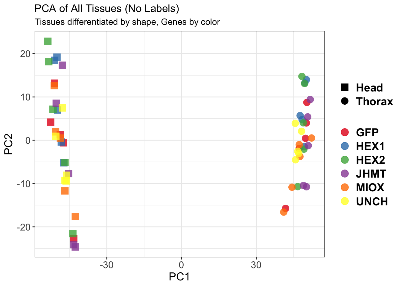
$WithLabel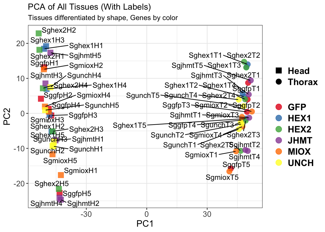
The PCA plot shows clear distinction between tissue types, while gene silencing has a large variation within each tissue, and presents no distinct clear groupings for a single gene.
SVA
### SVA analysis to control for technical variation
dat <- counts(dds, normalized = TRUE)
idx <- rowMeans(dat) > 1
dat <- dat[idx, ]
mod <- model.matrix(~ Gene, colData(dds))
mod0 <- model.matrix(~ 1, colData(dds))
svseq <- svaseq(dat, mod, mod0)Number of significant surrogate variables is: 3
Iteration (out of 5 ):1 2 3 4 5 sva_plots <- create_sva_plots(svseq, dds, saveDir, intgroup = c("Tissue", "Gene"))
# Show stripcharts in the report
sva_plots$Stripcharts[[1]] # Show first stripchart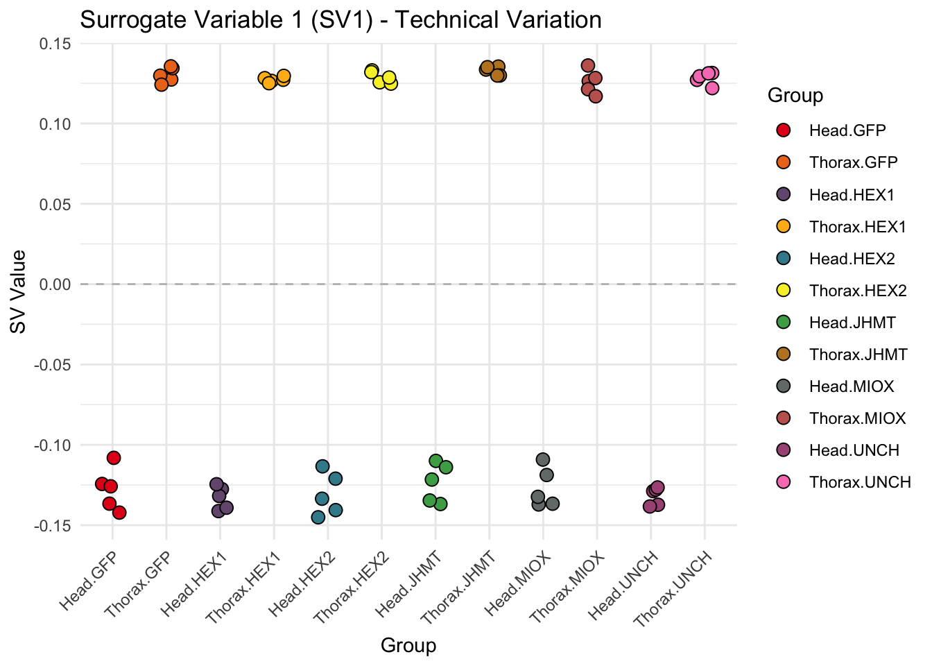
sva_plots$Stripcharts[[2]] # Show second stripchart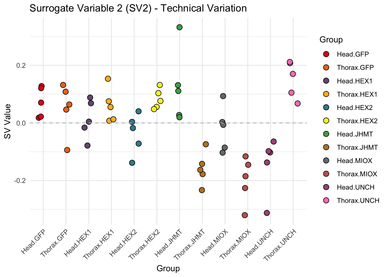
sva_plots$Stripcharts[[3]] # Show third stripchart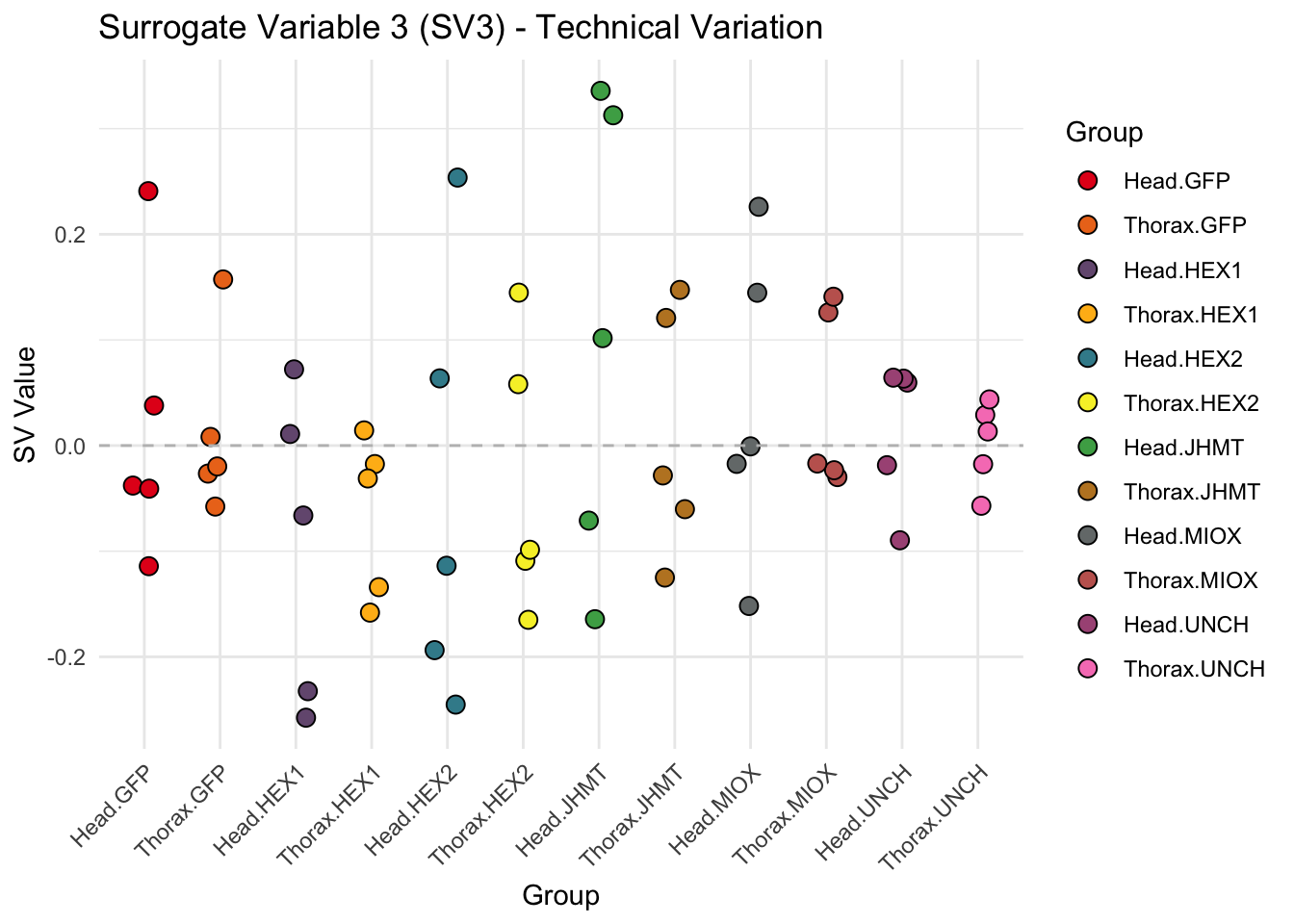
# Show scatter plots in the report
sva_plots$ScatterPlots[["1_2"]] # Show SV1 vs SV2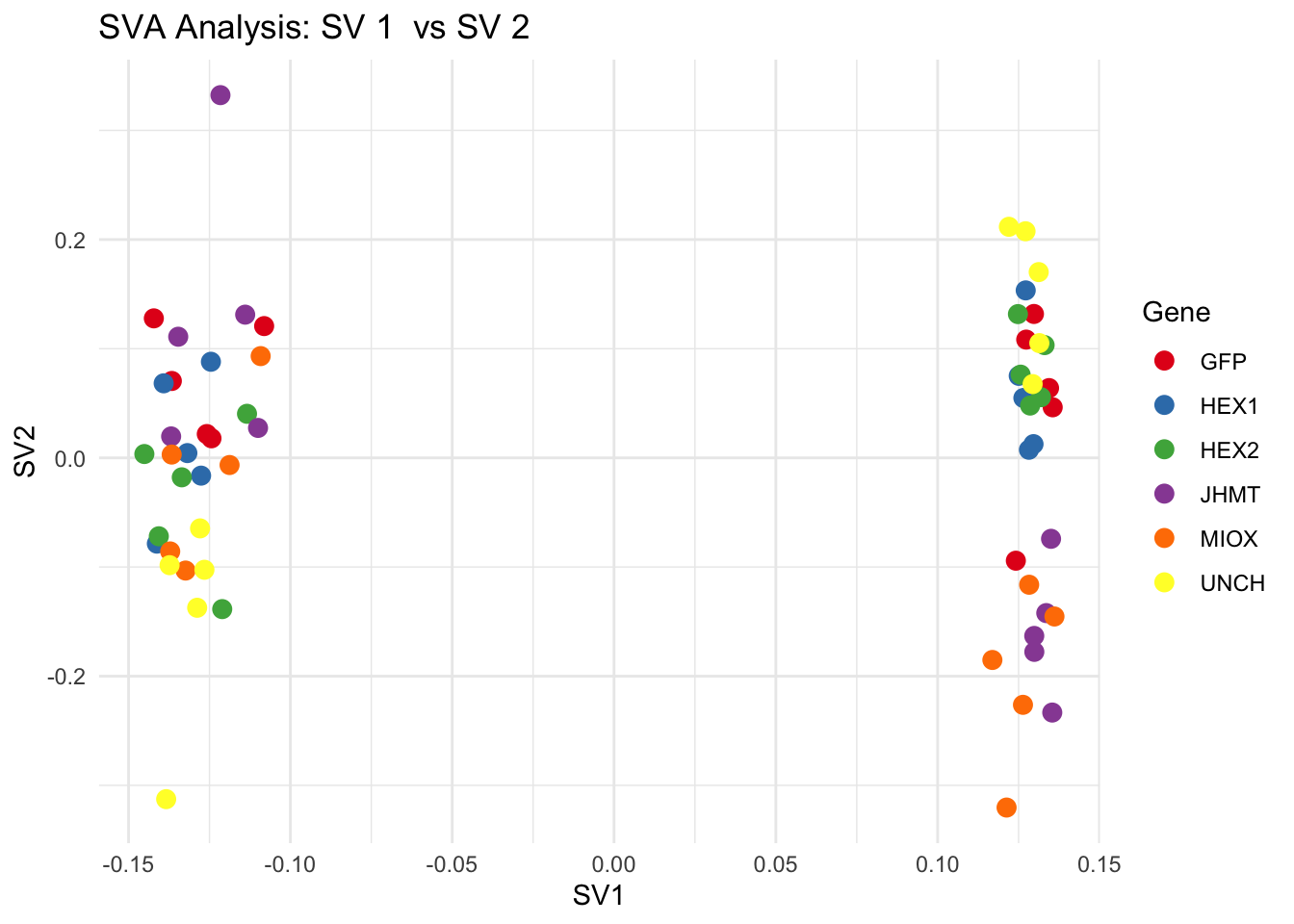
sva_plots$ScatterPlots[["1_3"]] # Show SV1 vs SV3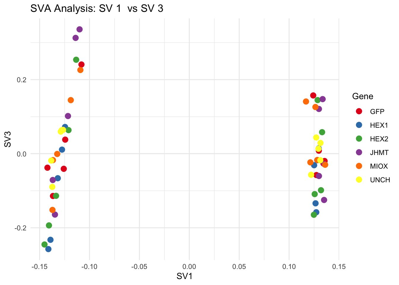
sva_plots$ScatterPlots[["2_3"]] # Show SV2 vs SV3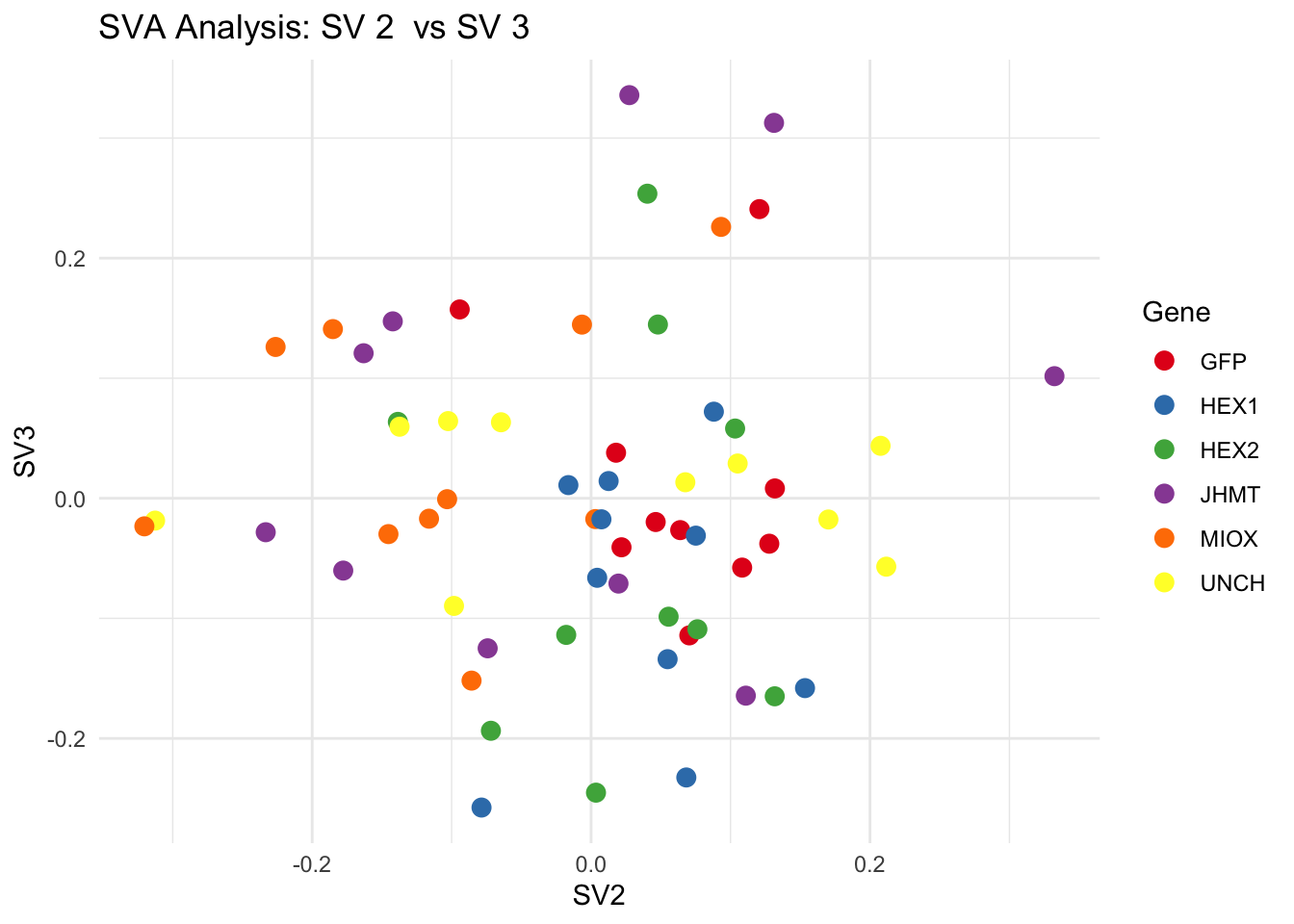
SV1 is clearly showing an effect of tissue. We rerun the
DESeq2 model but this time including the surrogate variable
SV2 and SV3 as a covariates only, as we know that the modeled variation
is more likely explained by tissue and gene variation rather than batch
effects.
ddssva <- dds
ddssva$SV2 <- svseq$sv[,2]
ddssva$SV3 <- svseq$sv[,3]
design(ddssva) <- ~ SV2 + SV3 + Gene
ddssva$Gene <- relevel(ddssva$Gene, ref = "GFP")
smallestGroupSize <- 5
keep <- rowSums(counts(ddssva) >= 10) >= smallestGroupSize
ddssva <- ddssva[keep,]
ddssva <- DESeq(ddssva)
ddssva <- ddssva[which(mcols(ddssva)$betaConv),] # remove non converging rows
### Extract results
message("Available contrasts are: ", paste(resultsNames(ddssva), collapse = ", "))
hex1 <- results(ddssva, name = "Gene_HEX1_vs_GFP", alpha = 0.05)
hex2 <- results(ddssva, name = "Gene_HEX2_vs_GFP", alpha = 0.05)
jhmt <- results(ddssva, name = "Gene_JHMT_vs_GFP", alpha = 0.05)
miox <- results(ddssva, name = "Gene_MIOX_vs_GFP", alpha = 0.05)
unch <- results(ddssva, name = "Gene_UNCH_vs_GFP", alpha = 0.05)Volcano plots and Heatmaps
# Define contrast_sets
hex1_samples <- c("SggfpH1","SggfpH2","SggfpH3","SggfpH4","SggfpH5",
"Sghex1H1","Sghex1H2","Sghex1H3","Sghex1H4","Sghex1H5",
"SggfpT1","SggfpT2","SggfpT3","SggfpT4","SggfpT5",
"Sghex1T1","Sghex1T2","Sghex1T3","Sghex1T4","Sghex1T5")
hex2_samples <- c("SggfpH1","SggfpH2","SggfpH3","SggfpH4","SggfpH5",
"Sghex2H1","Sghex2H2","Sghex2H3","Sghex2H4","Sghex2H5",
"SggfpT1","SggfpT2","SggfpT3","SggfpT4","SggfpT5",
"Sghex2T1","Sghex2T2","Sghex2T3","Sghex2T4","Sghex2T5")
jhmt_samples <- c("SggfpH1","SggfpH2","SggfpH3","SggfpH4","SggfpH5",
"SgjhmtH1","SgjhmtH2","SgjhmtH3","SgjhmtH4","SgjhmtH5",
"SggfpT1","SggfpT2","SggfpT3","SggfpT4","SggfpT5",
"SgjhmtT1","SgjhmtT2","SgjhmtT3","SgjhmtT4","SgjhmtT5")
miox_samples <- c("SggfpH1","SggfpH2","SggfpH3","SggfpH4","SggfpH5",
"SgmioxH1","SgmioxH2","SgmioxH3","SgmioxH4","SgmioxH5",
"SggfpT1","SggfpT2","SggfpT3","SggfpT4","SggfpT5",
"SgmioxT1","SgmioxT2","SgmioxT3","SgmioxT4","SgmioxT5")
unch_samples <- c("SggfpH1","SggfpH2","SggfpH3","SggfpH4","SggfpH5",
"SgunchH1","SgunchH2","SgunchH3","SgunchH4","SgunchH5",
"SggfpT1","SggfpT2","SggfpT3","SggfpT4","SggfpT5",
"SgunchT1","SgunchT2","SgunchT3","SgunchT4","SgunchT5")
# Run full analysis
hex1_plots <- visualize_data(hex1, "HEX1_vs_GFP", hex1_samples)
hex2_plots <- visualize_data(hex2, "HEX2_vs_GFP", hex2_samples)
jhmt_plots <- visualize_data(jhmt, "JHMT_vs_GFP", jhmt_samples)
miox_plots <- visualize_data(miox, "MIOX_vs_GFP", miox_samples)
unch_plots <- visualize_data(unch, "UNCH_vs_GFP", unch_samples)
hex1_plots$volcano; hex1_plots$heatmap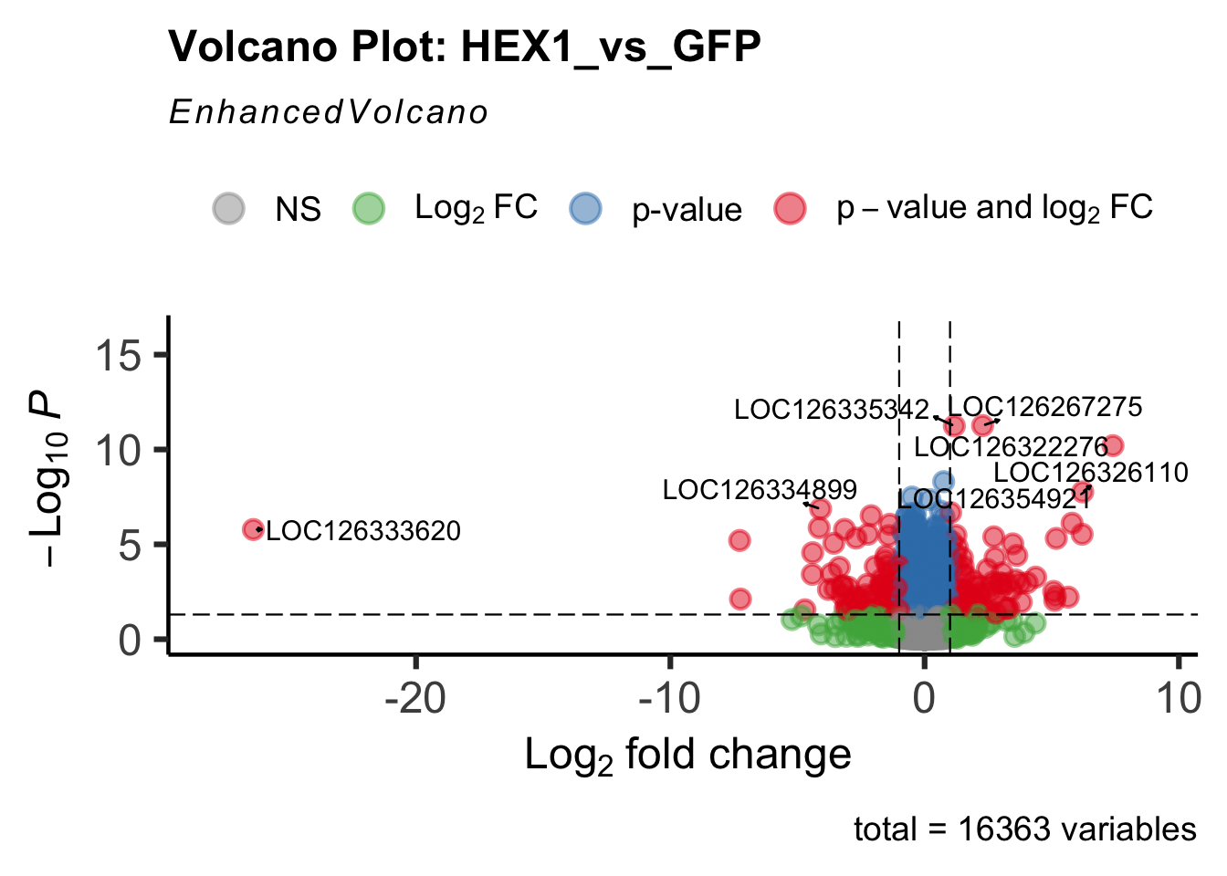
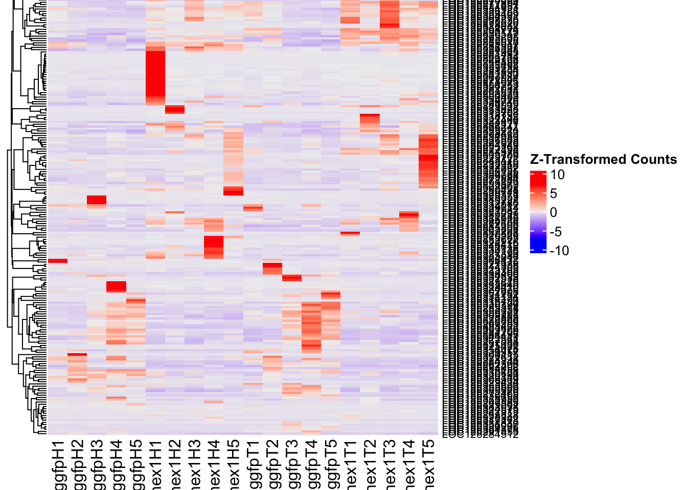
hex2_plots$volcano; hex2_plots$heatmap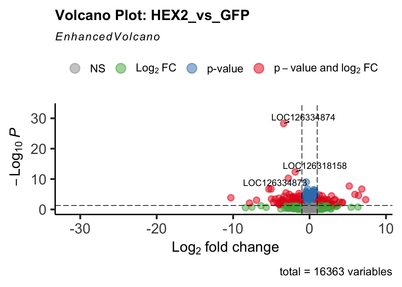
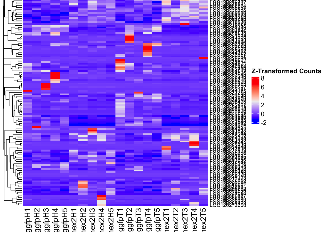
jhmt_plots$volcano; jhmt_plots$heatmap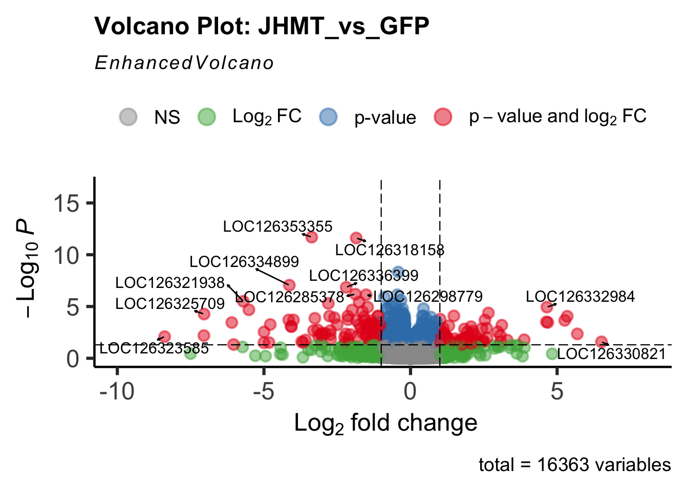
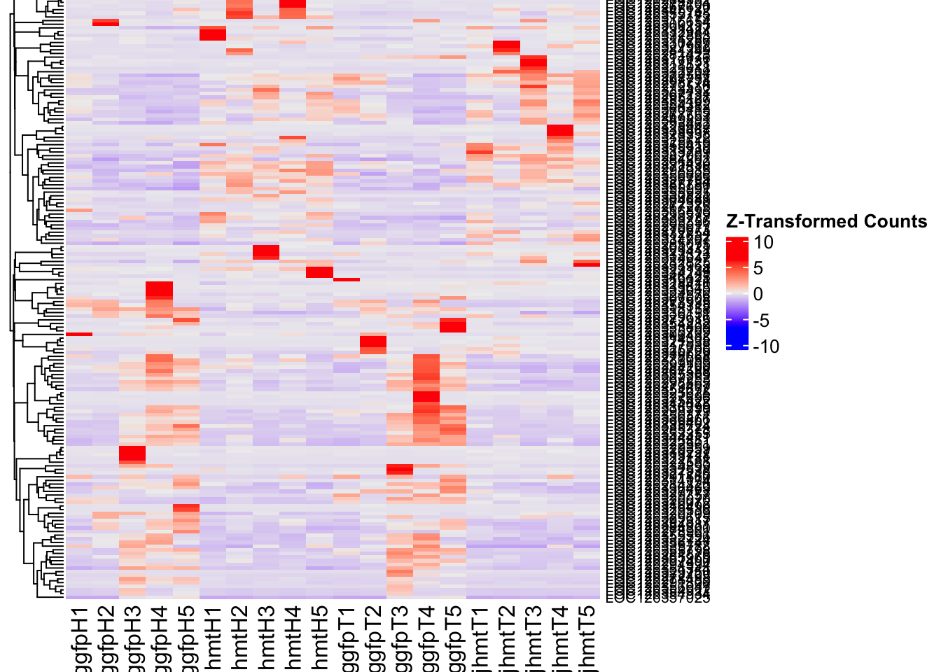
miox_plots$volcano; miox_plots$heatmap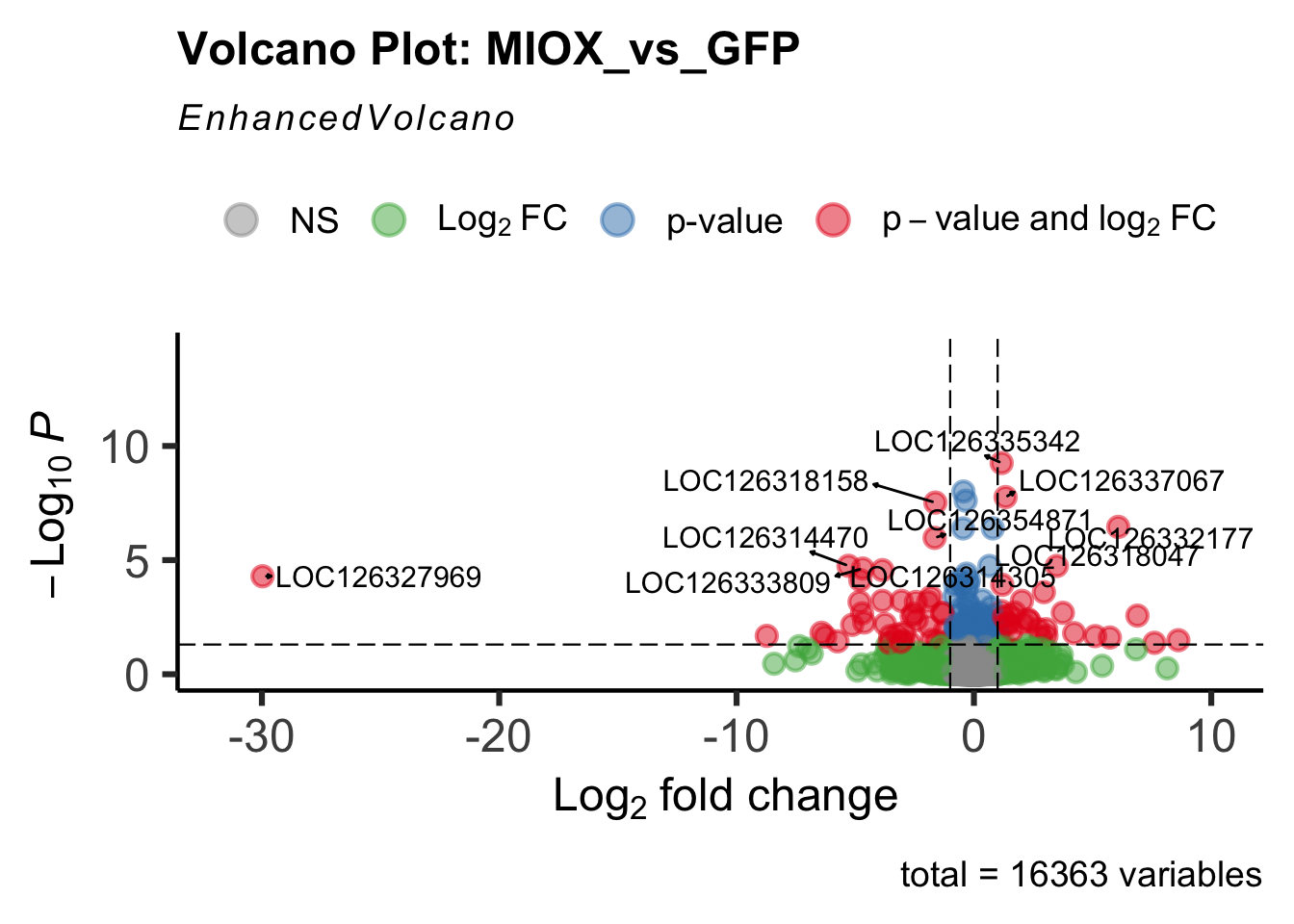
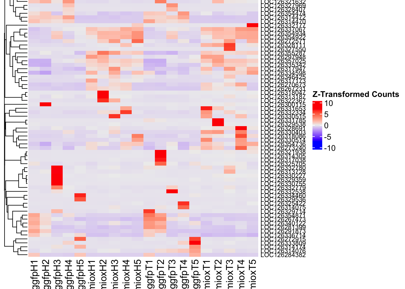
unch_plots$volcano; unch_plots$heatmap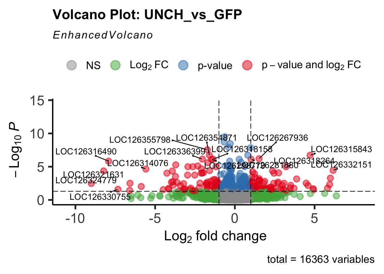
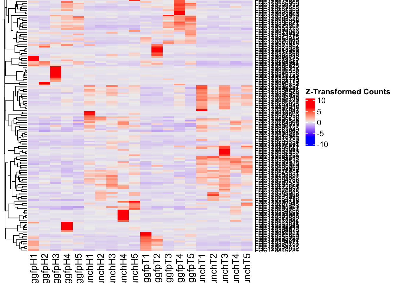
DEG tables
The following tables show the genes differentially expressed with at least an absolute log2fold change of > 1 considering all tissues together. Considering GFP as the reference state, upregulated genes in knockdown treatment in red and downregulated genes in knockdown treatment in blue. You can search for a gene of interest by writing a LOCID or description in the search bar or sort by column.
# Generate tables for each contrast
table_hex1 <- generate_deg_table(ddssva, "Gene_HEX1_vs_GFP", allspecies_df)
out of 16363 with nonzero total read count
adjusted p-value < 0.05
LFC > 0 (up) : 896, 5.5%
LFC < 0 (down) : 993, 6.1%
outliers [1] : 0, 0%
low counts [2] : 1269, 7.8%
(mean count < 9)
[1] see 'cooksCutoff' argument of ?results
[2] see 'independentFiltering' argument of ?resultsTotal DEGs p-value < 0.05 and absolute logFoldChange > 1: 205LFC > 1 (up) : 126 (61.46%)LFC < -1 (down) : 79 (38.54%)table_hex1$kable_tabletable_hex2 <- generate_deg_table(ddssva, "Gene_HEX2_vs_GFP", allspecies_df)
out of 16363 with nonzero total read count
adjusted p-value < 0.05
LFC > 0 (up) : 522, 3.2%
LFC < 0 (down) : 541, 3.3%
outliers [1] : 0, 0%
low counts [2] : 1587, 9.7%
(mean count < 11)
[1] see 'cooksCutoff' argument of ?results
[2] see 'independentFiltering' argument of ?resultsTotal DEGs p-value < 0.05 and absolute logFoldChange > 1: 121LFC > 1 (up) : 57 (47.11%)LFC < -1 (down) : 64 (52.89%)table_hex2$kable_tabletable_jhmt <- generate_deg_table(ddssva, "Gene_JHMT_vs_GFP", allspecies_df)
out of 16363 with nonzero total read count
adjusted p-value < 0.05
LFC > 0 (up) : 371, 2.3%
LFC < 0 (down) : 672, 4.1%
outliers [1] : 0, 0%
low counts [2] : 318, 1.9%
(mean count < 6)
[1] see 'cooksCutoff' argument of ?results
[2] see 'independentFiltering' argument of ?resultsTotal DEGs p-value < 0.05 and absolute logFoldChange > 1: 174LFC > 1 (up) : 82 (47.13%)LFC < -1 (down) : 92 (52.87%)table_jhmt$kable_tabletable_miox <- generate_deg_table(ddssva, "Gene_MIOX_vs_GFP", allspecies_df)
out of 16363 with nonzero total read count
adjusted p-value < 0.05
LFC > 0 (up) : 71, 0.43%
LFC < 0 (down) : 131, 0.8%
outliers [1] : 0, 0%
low counts [2] : 0, 0%
(mean count < 1)
[1] see 'cooksCutoff' argument of ?results
[2] see 'independentFiltering' argument of ?resultsTotal DEGs p-value < 0.05 and absolute logFoldChange > 1: 69LFC > 1 (up) : 31 (44.93%)LFC < -1 (down) : 38 (55.07%)table_miox$kable_tabletable_unch <- generate_deg_table(ddssva, "Gene_UNCH_vs_GFP", allspecies_df)
out of 16363 with nonzero total read count
adjusted p-value < 0.05
LFC > 0 (up) : 213, 1.3%
LFC < 0 (down) : 337, 2.1%
outliers [1] : 0, 0%
low counts [2] : 0, 0%
(mean count < 1)
[1] see 'cooksCutoff' argument of ?results
[2] see 'independentFiltering' argument of ?resultsTotal DEGs p-value < 0.05 and absolute logFoldChange > 1: 155LFC > 1 (up) : 80 (51.61%)LFC < -1 (down) : 75 (48.39%)table_unch$kable_tableSummary and Overlap
# Summarize DEGs for all contrasts
deg_summary <- bind_rows(
summarize_deg_counts(table_hex1, "HEX1 vs GFP"),
summarize_deg_counts(table_hex2, "HEX2 vs GFP"),
summarize_deg_counts(table_jhmt, "JHMT vs GFP"),
summarize_deg_counts(table_miox, "MIOX vs GFP"),
summarize_deg_counts(table_unch, "UNCH vs GFP")
)
# Display table using kable with styling
deg_summary %>%
kable("html", escape = FALSE, col.names = gsub("_", " ", names(.))) %>%
kable_styling("striped", full_width = TRUE) %>%
column_spec(2, color = "red", bold = TRUE) %>% # Upregulated in red
column_spec(3, color = "blue", bold = TRUE) %>% # Downregulated in blue
add_header_above(c("Summary of DEGs" = 3)) %>%
row_spec(0, bold = TRUE)| Contrast | Upregulated | Downregulated |
|---|---|---|
| HEX1 vs GFP | 123 | 78 |
| HEX2 vs GFP | 51 | 64 |
| JHMT vs GFP | 77 | 89 |
| MIOX vs GFP | 30 | 38 |
| UNCH vs GFP | 76 | 74 |
# Define the list of RNAi contrasts
contrast_list <- c("HEX1_vs_GFP", "HEX2_vs_GFP", "JHMT_vs_GFP",
"MIOX_vs_GFP", "UNCH_vs_GFP")
# Initialize empty lists for storing Head-specific DEGs for each contrast
venn_data_up <- list()
venn_data_down <- list()
venn_data_all <- list()
# Function to load Head-specific DEGs for a given set of contrasts
load_deg_contrasts_head <- function(contrast_list) {
degs_up <- list()
degs_down <- list()
degs_all <- list()
for (contrast in contrast_list) {
deg_file <- file.path(workDir, "DEG_results/RNAi/All/", contrast, paste0("DEG_sigresults_", contrast, ".csv"))
if (!file.exists(deg_file)) {
message(paste("File missing for contrast:", contrast))
next # Skip if the file doesn't exist
}
deg_data <- read.csv(deg_file, stringsAsFactors = FALSE)
# Convert row names to a column if necessary
if ("X" %in% colnames(deg_data)) {
colnames(deg_data)[colnames(deg_data) == "X"] <- "GeneID"
}
# Check if data is empty
if (nrow(deg_data) == 0) {
message(paste("No data for contrast:", contrast))
next
}
# Select significant DEGs (Up, Down, All)
degs_up[[contrast]] <- deg_data %>%
filter(padj < 0.05 & log2FoldChange >= 1) %>%
pull(GeneID) # Extract GeneID column
degs_down[[contrast]] <- deg_data %>%
filter(padj < 0.05 & log2FoldChange <= -1) %>%
pull(GeneID) # Extract GeneID column
degs_all[[contrast]] <- deg_data %>%
filter(padj < 0.05 & abs(log2FoldChange) >= 1) %>%
pull(GeneID) # Extract GeneID column
}
return(list(up = degs_up, down = degs_down, all = degs_all))
}
# Load DEG data for the defined contrasts (Head tissue only)
venn_data_contrasts <- load_deg_contrasts_head(contrast_list)
# Prepare the data for the Venn diagrams
venn_data_up <- venn_data_contrasts$up
venn_data_down <- venn_data_contrasts$down
venn_data_all <- venn_data_contrasts$all
# Function to display Venn diagram and corresponding datatable
display_venn_with_datatable <- function(venn_data, title, allspecies_df) {
# Calculate the overlapping genes
overlap_genes <- Reduce(intersect, venn_data)
# Create a data frame for the overlapping genes
overlap_df <- data.frame(GeneID = overlap_genes)
# Merge to get species information
meta_brock_df <- merge(overlap_df, allspecies_df, by = "GeneID", all.x = TRUE)
# Generate the Venn diagram
venn_plot <- venn.diagram(
x = venn_data,
category.names = contrast_list,
filename = NULL,
output = TRUE,
fill = c("orange", "red", "blue", "purple", "green"), # Adjust colors for contrasts
alpha = 0.5,
cex = 2,
cat.cex = 0,
main = title,
main.cex = 1.2
)
# Clear the plotting area before drawing
grid.newpage()
grid.draw(venn_plot)
# Create a custom legend
legend_labels <- contrast_list
legend_colors <- c("orange", "red", "blue", "purple", "green")
# Positioning the legend
legend_x <- unit(0.85, "npc") # Adjust x position
legend_y <- unit(0.2, "npc") # Adjust y position
# Draw the legend
for (i in 1:length(legend_labels)) {
grid.rect(x = legend_x, y = legend_y - unit((i - 1) * 0.05, "npc"),
width = unit(0.02, "npc"), height = unit(0.02, "npc"),
gp = gpar(fill = legend_colors[i], col = NA))
grid.text(label = legend_labels[i], x = legend_x + unit(0.05, "npc"),
y = legend_y - unit((i - 1) * 0.05, "npc"),
just = "left", gp = gpar(cex = 0.8))
}
# Display the merged overlapping genes table with datatable
datatable(meta_brock_df, options = list(
pageLength = 10,
scrollX = TRUE,
autoWidth = TRUE,
searchHighlight = TRUE
),
rownames = FALSE,
escape = FALSE
) %>%
formatStyle(
'Species', target = 'cell',
fontStyle = 'italic'
) %>%
formatStyle(
columns = names(meta_brock_df),
target = 'row',
color = styleEqual(c("red", "blue", "black"), c("red", "blue", "black")),
fontWeight = styleEqual(c("bold", "normal"), c("bold", "normal")),
backgroundColor = styleEqual(c("red", "blue", "black"), c("white", "white", "white"))
)
}
# Display the Venn diagram and datatable for **Head Upregulated DEGs** across contrasts
display_venn_with_datatable(venn_data_up, "Venn Diagram of Head Upregulated DEGs - RNAi Contrasts", allspecies_df)
| Version | Author | Date |
|---|---|---|
| b540a1e | Maeva TECHER | 2025-02-27 |
# Display the Venn diagram and datatable for **Head Downregulated DEGs** across contrasts
display_venn_with_datatable(venn_data_down, "Venn Diagram of Head Downregulated DEGs - RNAi Contrasts", allspecies_df)
| Version | Author | Date |
|---|---|---|
| b540a1e | Maeva TECHER | 2025-02-27 |
# Display the Venn diagram and datatable for **All Significant DEGs in Head Tissue**
display_venn_with_datatable(venn_data_all, "Venn Diagram of All Significant DEGs in Head Tissue - RNAi Contrasts", allspecies_df)
| Version | Author | Date |
|---|---|---|
| b540a1e | Maeva TECHER | 2025-02-27 |
Head tissue
Minor changes here are made compared to the DESeq2 results regarding the importation of samples to transform into a matrix. Sample names are structured as follow: {Sg}{gene}{#} {Sg} = Schistocerca gregaria {gene} = gene abbreviation gfp, hex1, hex2, jhmt, miox and unch H{#} = biological replicate
saveDir <- paste0(workDir,"/DEG_results/RNAi/Head")
dir.create(saveDir)
### Prepare Sample CSV file #####
samples <- read.delim(file.path(workDir, "list/RNAi/Head_RNAisample_list.csv"), sep = ",", row.names = 1, header = TRUE)
files <- file.path(workDir, "readcounts/RNAi/", samples$Tissue, samples$Filename)
names(files) <- row.names(samples)
if (all(file.exists(files))) {
message("All the files exist!")
} else {
warning("Some files are missing!")
}All the files exist!### Create count sample matrix
cts <- map_dfc(files, function(sample) {
data_count <- read.delim(sample, sep = "\t", header = FALSE)
col_name <- gsub("_counts.txt", "", basename(sample))
setNames(data.frame(data_count[, 2]), col_name)
})
row_get <- read.delim(files[1], sep = "\t", row.names = 1, header = F) # Get proper row names
rownames(cts) <- rownames(row_get)
rm(row_get) # remove unused object from memoryWhile for bulk RNAseq on head and thorax for all species, the DEGs model was made between isolated and crowded individuals (with isolated as the reference state), here, the DEG analysis will be carried between GFP knock-down nymphs (as reference state) vs Hexamerins / Juvenile Hormones / Uncharacterized proteins.
### Build DESeq2 Object
dds <- DESeqDataSetFromMatrix(countData = cts,
colData = samples,
design = ~ Gene)
dds$Gene <- relevel(dds$Gene, ref = "GFP")
smallestGroupSize <- 5
keep <- rowSums(counts(dds) >= 10) >= smallestGroupSize
dds <- dds[keep,]
dds <- DESeq(dds)Normalization and PCA
# Plot PCA and investigate quality metrics
vsd <- vst(dds, blind=T)
pca_results <- create_pca_plots(norm.dds = vsd, saveDir, transformation = "vst", intgroup = "Gene")
pca_results$PCA_Labelled
pca_results$PCA_Hull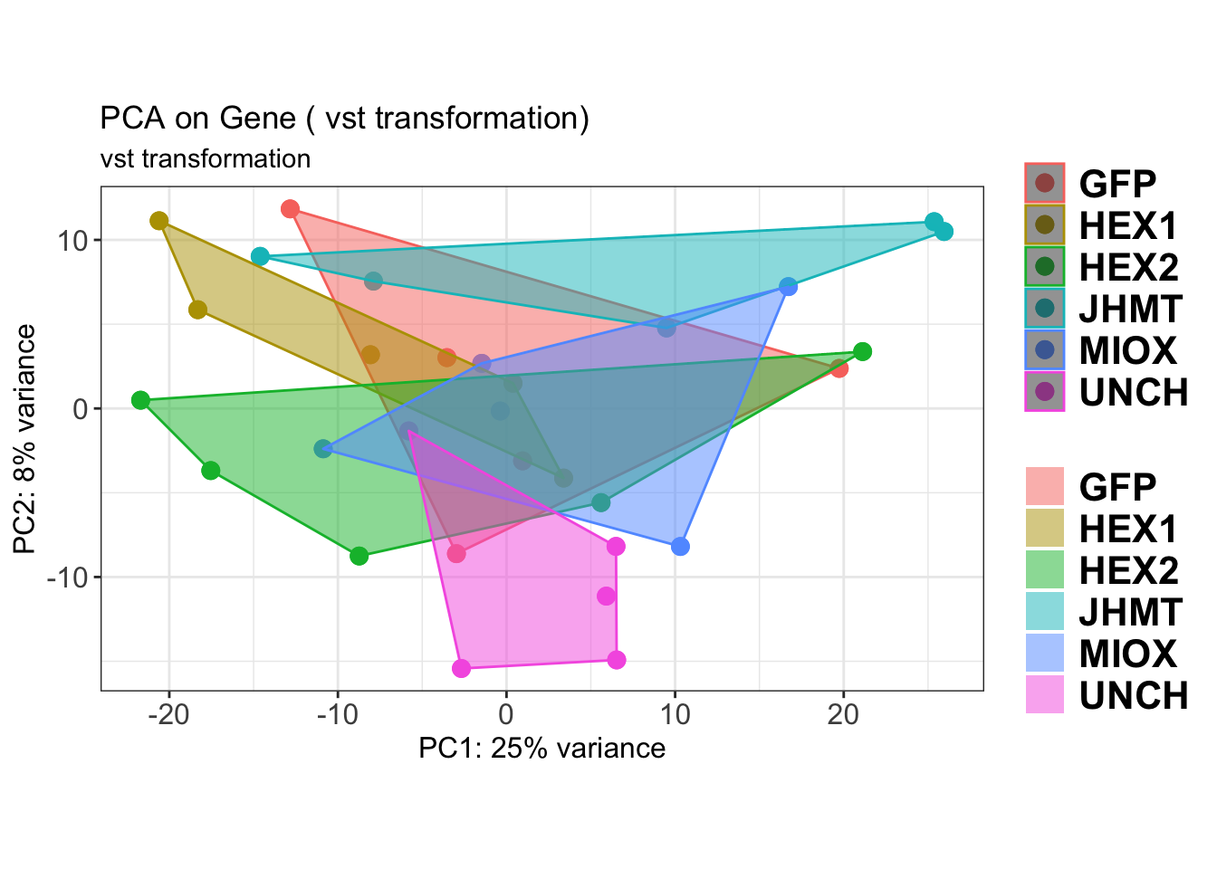
SVA
### SVA analysis to control for technical variation
dat <- counts(dds, normalized = TRUE)
idx <- rowMeans(dat) > 1
dat <- dat[idx, ]
mod <- model.matrix(~ Gene, colData(dds))
mod0 <- model.matrix(~ 1, colData(dds))
svseq <- svaseq(dat, mod, mod0)Number of significant surrogate variables is: 3
Iteration (out of 5 ):1 2 3 4 5 sva_plots <- create_sva_plots(svseq, dds, saveDir, intgroup = c("Tissue", "Gene"))
# Show stripcharts in the report
sva_plots$Stripcharts[[1]] # Show first stripchart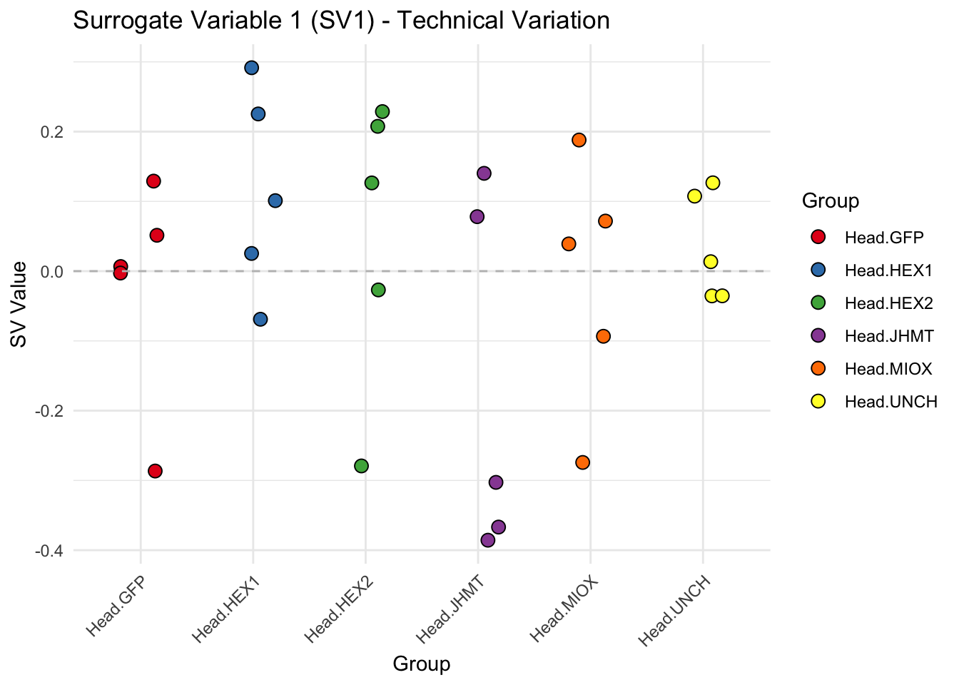
sva_plots$Stripcharts[[2]] # Show second stripchart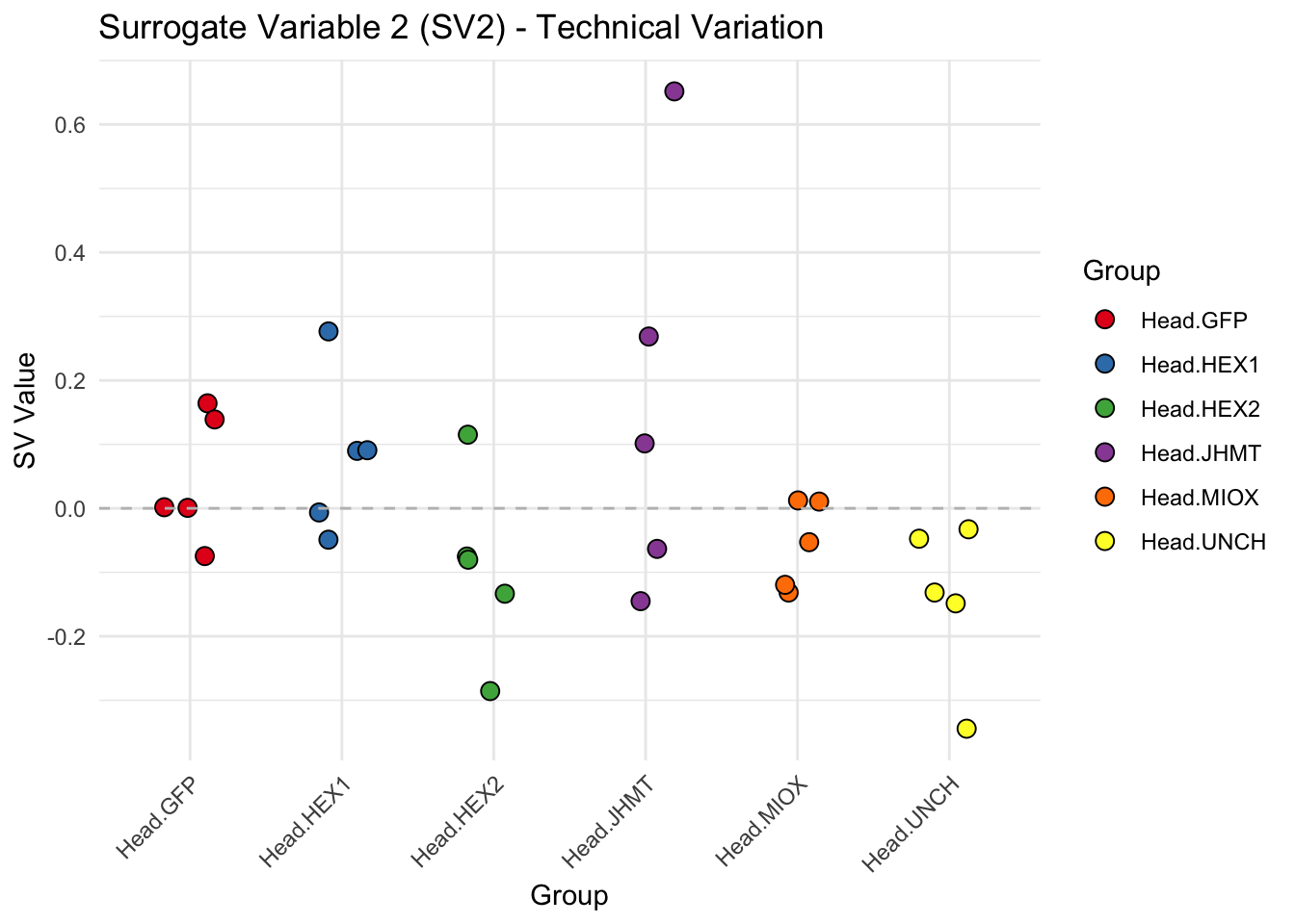
sva_plots$Stripcharts[[3]] # Show third stripchart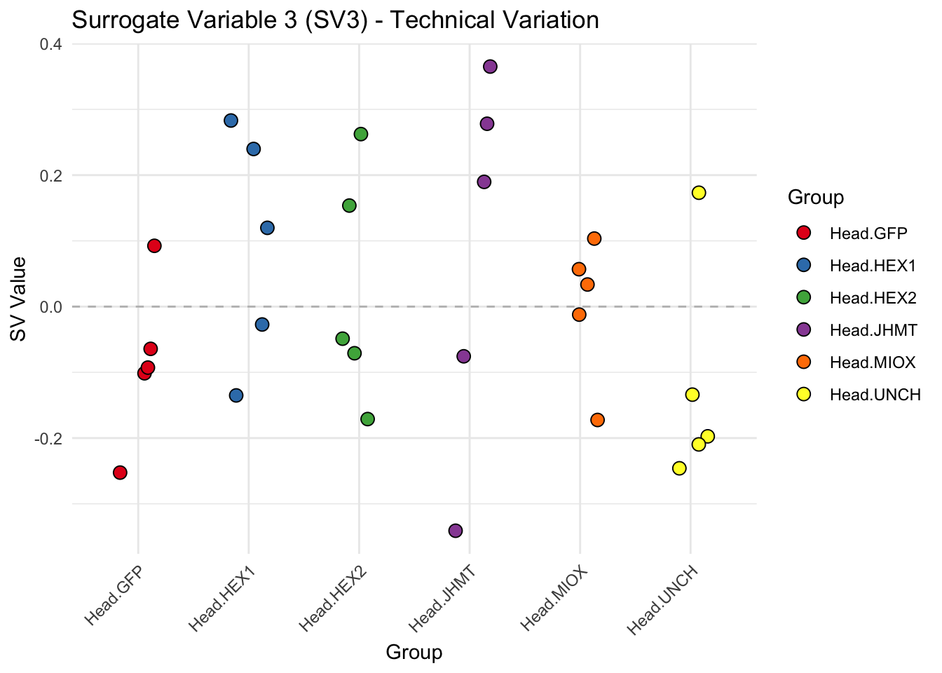
| Version | Author | Date |
|---|---|---|
| d7fa779 | Maeva TECHER | 2025-02-14 |
# Show scatter plots in the report
sva_plots$ScatterPlots[["1_2"]] # Show SV1 vs SV2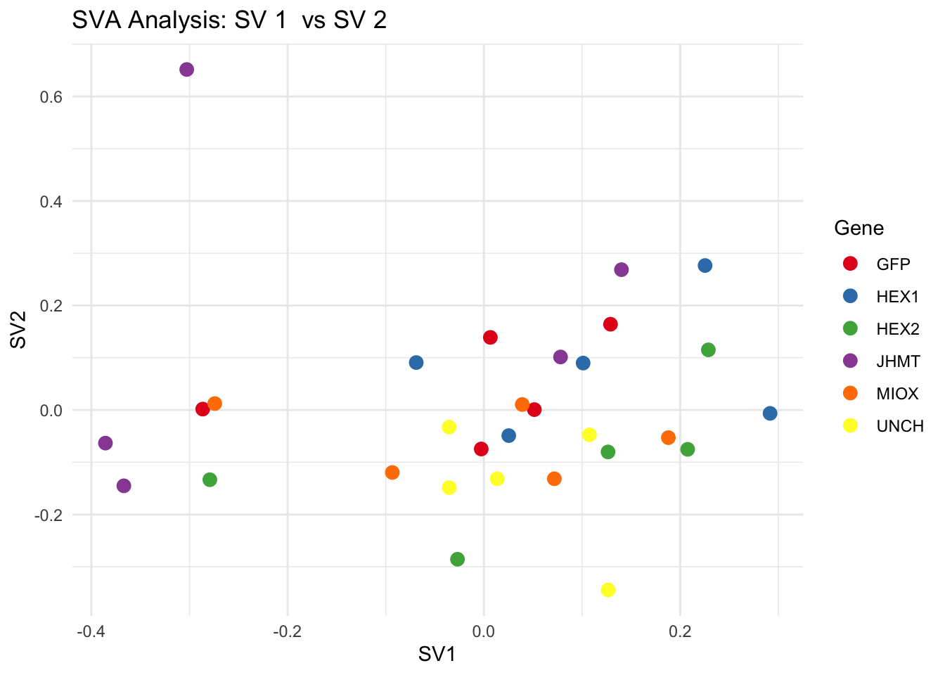
sva_plots$ScatterPlots[["1_3"]] # Show SV1 vs SV3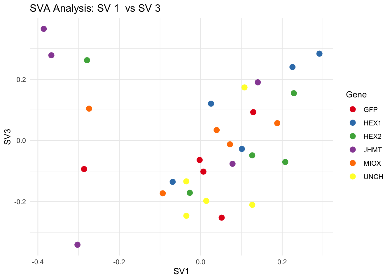
sva_plots$ScatterPlots[["2_3"]] # Show SV2 vs SV3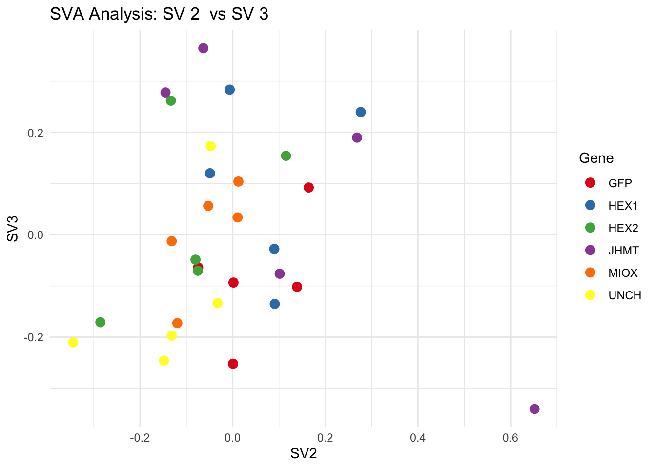
| Version | Author | Date |
|---|---|---|
| d7fa779 | Maeva TECHER | 2025-02-14 |
We rerun the DESeq2 model but this time including the
surrogate variable as a covariate, as we know that the modeled variation
is more likely explained by tissue and gene variation rather than batch
effects.
ddssva <- dds
ddssva$SV1 <- svseq$sv[,1]
ddssva$SV2 <- svseq$sv[,2]
ddssva$SV3 <- svseq$sv[,3]
design(ddssva) <- ~ SV1 + SV2 + SV3 + Gene
ddssva$Gene <- relevel(ddssva$Gene, ref = "GFP")
smallestGroupSize <- 5
keep <- rowSums(counts(ddssva) >= 10) >= smallestGroupSize
ddssva <- ddssva[keep,]
ddssva <- DESeq(ddssva)
ddssva <- ddssva[which(mcols(ddssva)$betaConv),] # remove non converging rows
### Extract results
message("Available contrasts are: ", paste(resultsNames(ddssva), collapse = ", "))
hex1 <- results(ddssva, name = "Gene_HEX1_vs_GFP", alpha = 0.05)
hex2 <- results(ddssva, name = "Gene_HEX2_vs_GFP", alpha = 0.05)
jhmt <- results(ddssva, name = "Gene_JHMT_vs_GFP", alpha = 0.05)
miox <- results(ddssva, name = "Gene_MIOX_vs_GFP", alpha = 0.05)
unch <- results(ddssva, name = "Gene_UNCH_vs_GFP", alpha = 0.05)Volcano plots and Heatmaps
First we create function to generate the plots we are interested to obtain and then run the whole pipeline for each gene.
# Define contrast_sets
hex1_samples <- c("SggfpH1","SggfpH2","SggfpH3","SggfpH4","SggfpH5",
"Sghex1H1","Sghex1H2","Sghex1H3","Sghex1H4","Sghex1H5")
hex2_samples <- c("SggfpH1","SggfpH2","SggfpH3","SggfpH4","SggfpH5",
"Sghex2H1","Sghex2H2","Sghex2H3","Sghex2H4","Sghex2H5")
jhmt_samples <- c("SggfpH1","SggfpH2","SggfpH3","SggfpH4","SggfpH5",
"SgjhmtH1","SgjhmtH2","SgjhmtH3","SgjhmtH4","SgjhmtH5")
miox_samples <- c("SggfpH1","SggfpH2","SggfpH3","SggfpH4","SggfpH5",
"SgmioxH1","SgmioxH2","SgmioxH3","SgmioxH4","SgmioxH5")
unch_samples <- c("SggfpH1","SggfpH2","SggfpH3","SggfpH4","SggfpH5",
"SgunchH1","SgunchH2","SgunchH3","SgunchH4","SgunchH5")
# Run full analysis
hex1_plots <- visualize_data(hex1, "HEX1_vs_GFP", hex1_samples)
hex2_plots <- visualize_data(hex2, "HEX2_vs_GFP", hex2_samples)
jhmt_plots <- visualize_data(jhmt, "JHMT_vs_GFP", jhmt_samples)
miox_plots <- visualize_data(miox, "MIOX_vs_GFP", miox_samples)
unch_plots <- visualize_data(unch, "UNCH_vs_GFP", unch_samples)
hex1_plots$volcano; hex1_plots$heatmap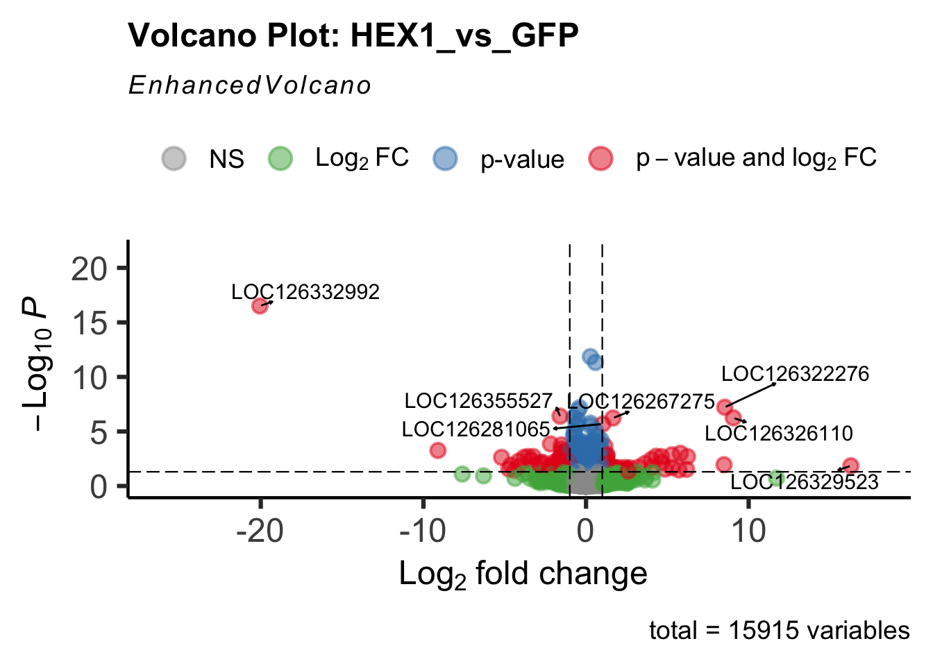
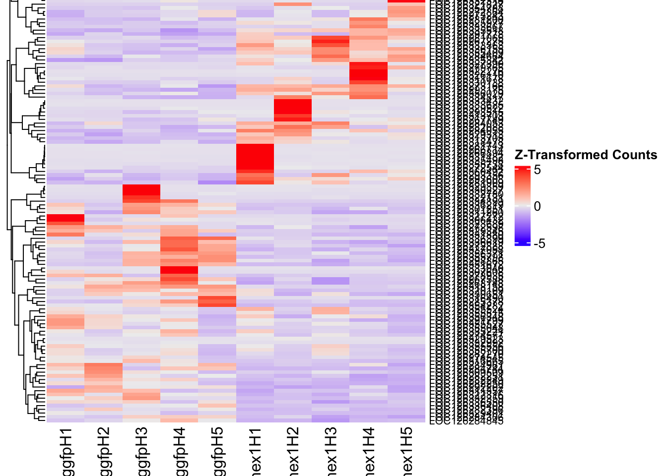
hex2_plots$volcano; hex2_plots$heatmap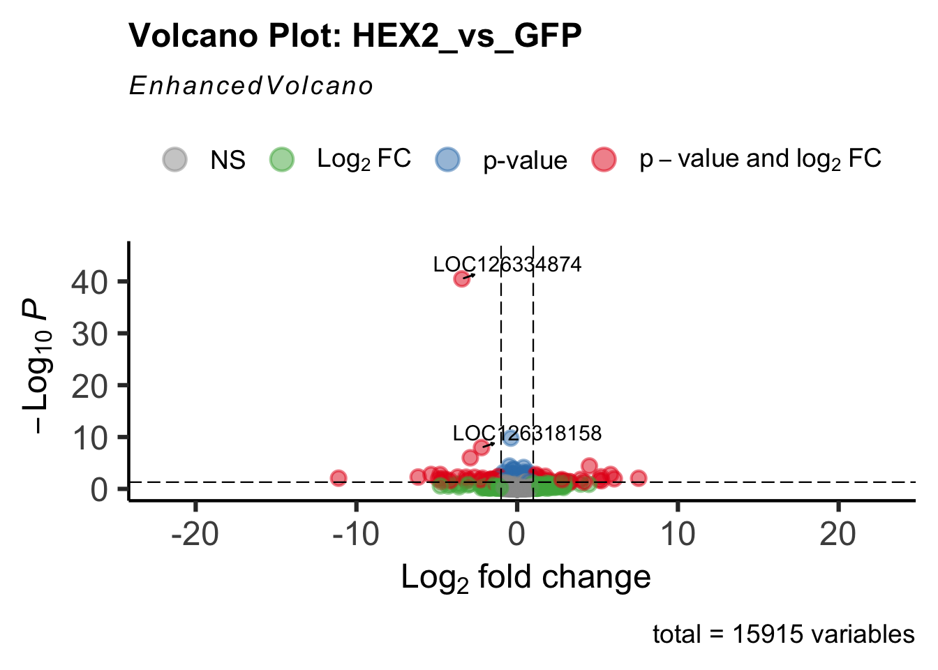
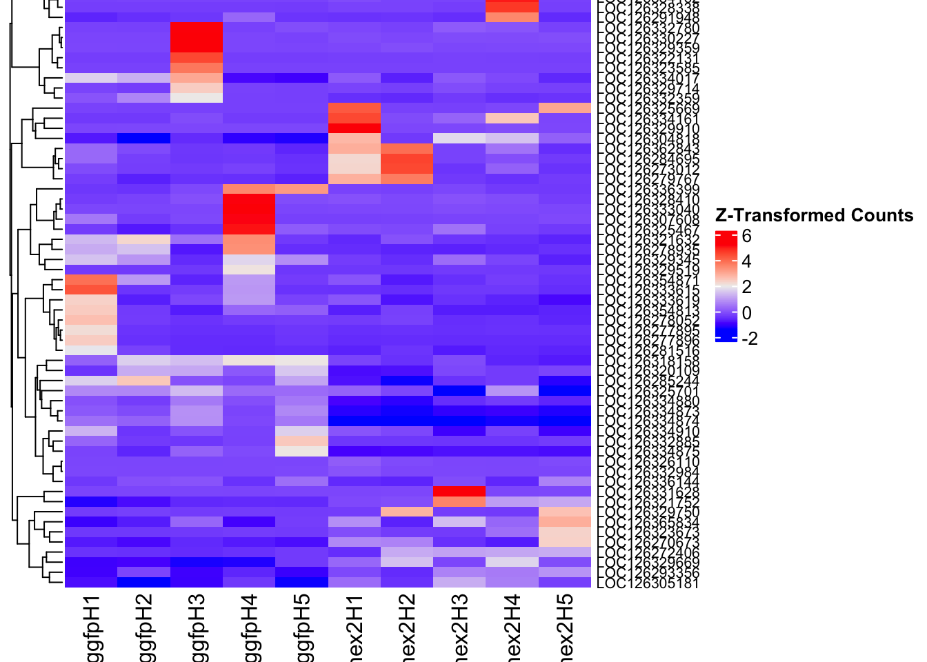
jhmt_plots$volcano; jhmt_plots$heatmap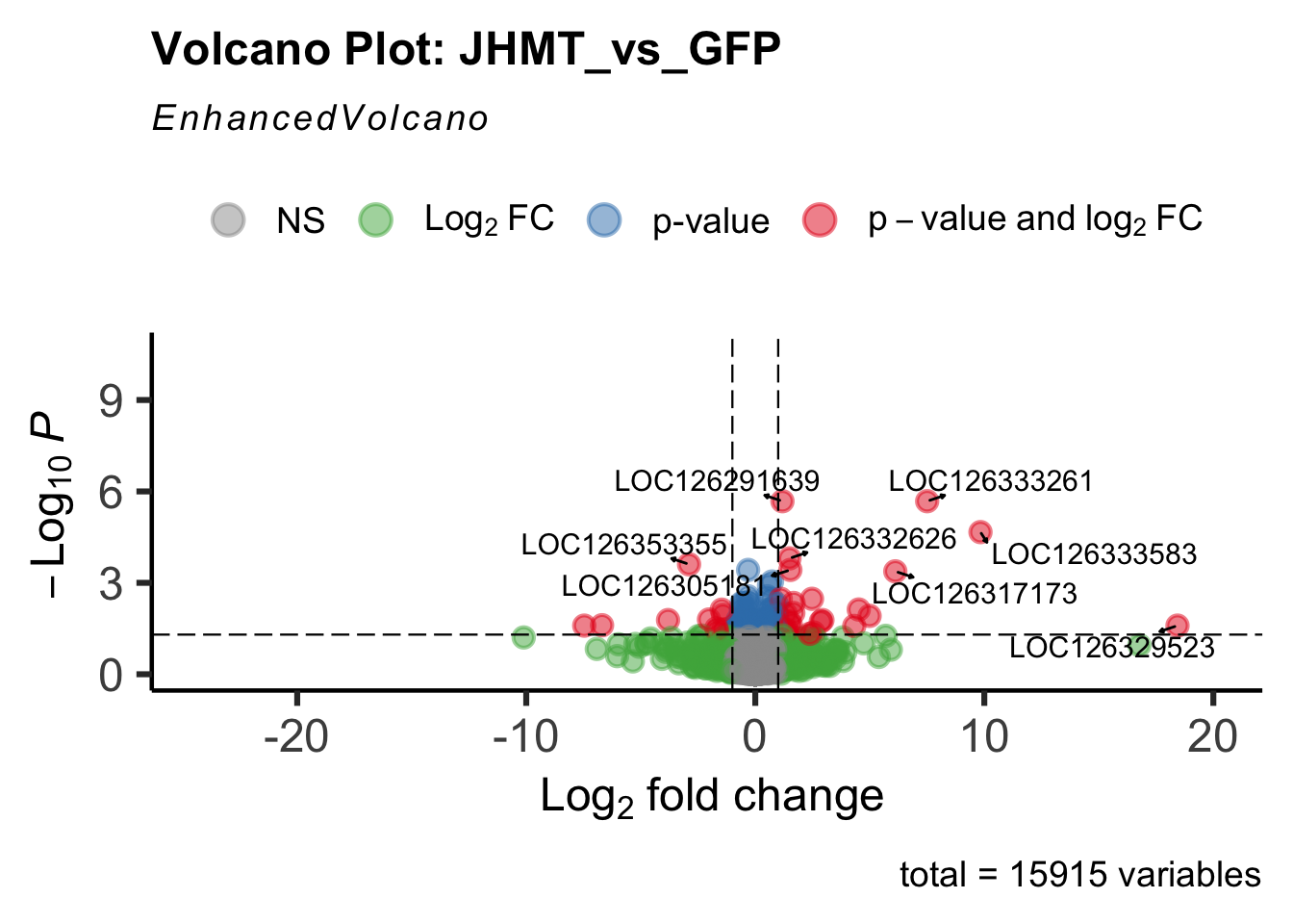
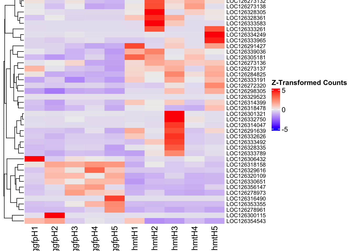
miox_plots$volcano; miox_plots$heatmap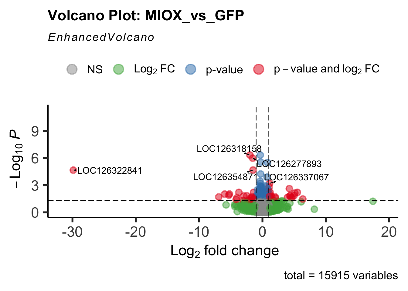
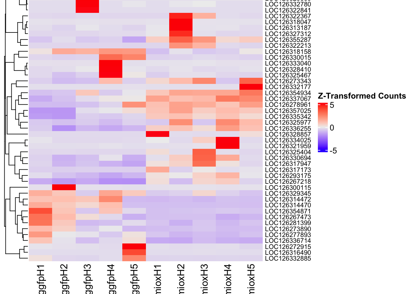
unch_plots$volcano; unch_plots$heatmap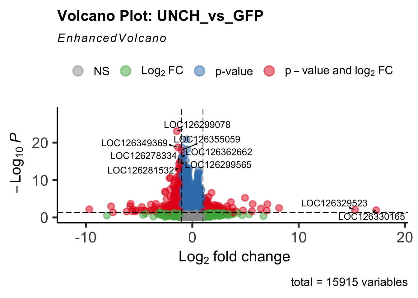
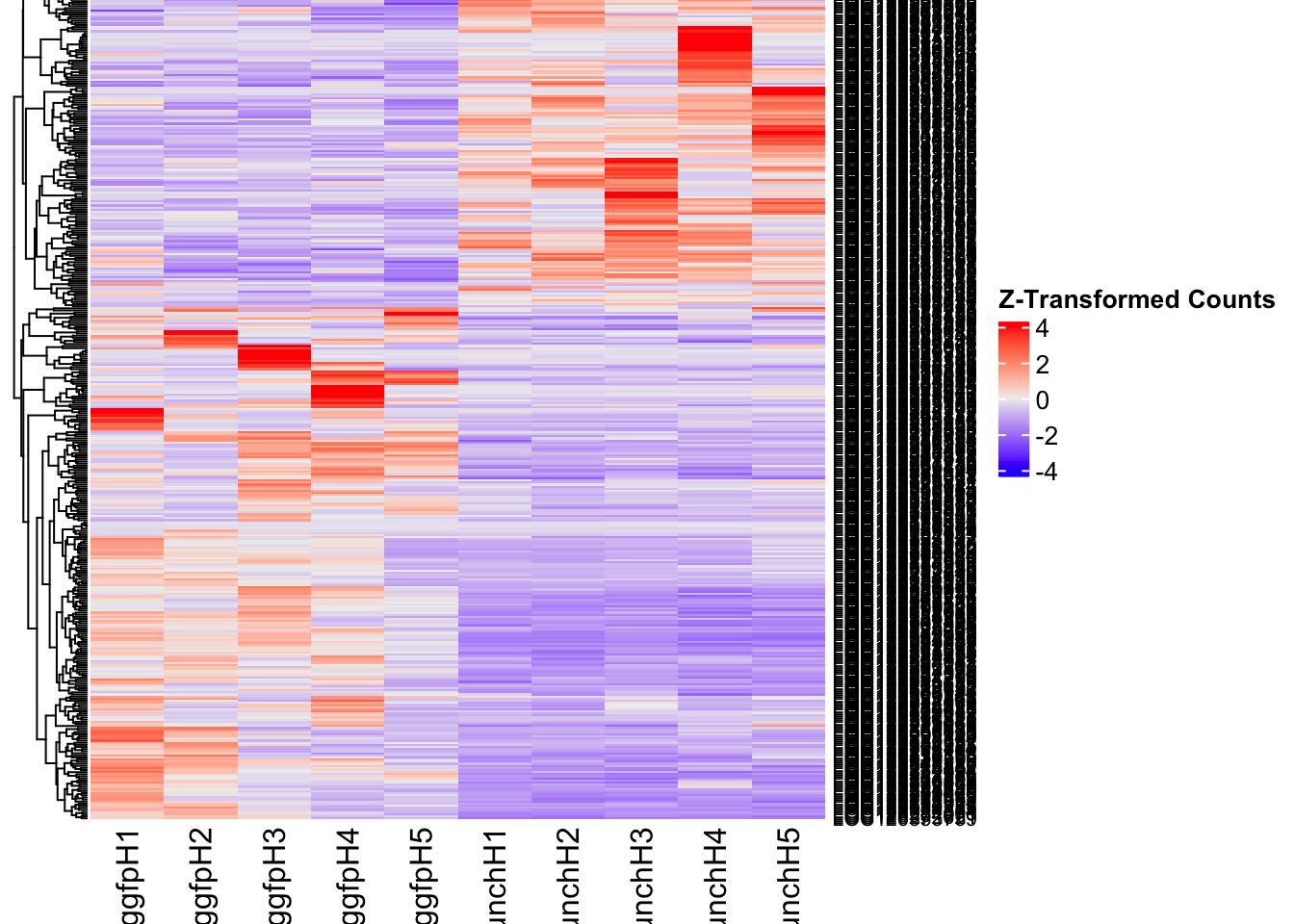
DEG tables
The following tables show the genes differentially expressed with at least an absolute log2fold change of > 1 considering head tissue only. Considering GFP as the reference state, upregulated genes in knockdown treatment in red and downregulated genes in knockdown treatment in blue. You can search for a gene of interest by writting a LOCID or description in the search bar or sort by column.
# Generate tables for each contrast
table_hex1 <- generate_deg_table(ddssva, "Gene_HEX1_vs_GFP", allspecies_df)
out of 15915 with nonzero total read count
adjusted p-value < 0.05
LFC > 0 (up) : 430, 2.7%
LFC < 0 (down) : 557, 3.5%
outliers [1] : 0, 0%
low counts [2] : 1852, 12%
(mean count < 17)
[1] see 'cooksCutoff' argument of ?results
[2] see 'independentFiltering' argument of ?resultsTotal DEGs p-value < 0.05 and absolute logFoldChange > 1: 121LFC > 1 (up) : 57 (47.11%)LFC < -1 (down) : 64 (52.89%)table_hex1$kable_tabletable_hex2 <- generate_deg_table(ddssva, "Gene_HEX2_vs_GFP", allspecies_df)
out of 15915 with nonzero total read count
adjusted p-value < 0.05
LFC > 0 (up) : 143, 0.9%
LFC < 0 (down) : 370, 2.3%
outliers [1] : 0, 0%
low counts [2] : 4011, 25%
(mean count < 50)
[1] see 'cooksCutoff' argument of ?results
[2] see 'independentFiltering' argument of ?resultsTotal DEGs p-value < 0.05 and absolute logFoldChange > 1: 62LFC > 1 (up) : 25 (40.32%)LFC < -1 (down) : 37 (59.68%)table_hex2$kable_tabletable_jhmt <- generate_deg_table(ddssva, "Gene_JHMT_vs_GFP", allspecies_df)
out of 15915 with nonzero total read count
adjusted p-value < 0.05
LFC > 0 (up) : 79, 0.5%
LFC < 0 (down) : 104, 0.65%
outliers [1] : 0, 0%
low counts [2] : 1543, 9.7%
(mean count < 14)
[1] see 'cooksCutoff' argument of ?results
[2] see 'independentFiltering' argument of ?resultsTotal DEGs p-value < 0.05 and absolute logFoldChange > 1: 42LFC > 1 (up) : 30 (71.43%)LFC < -1 (down) : 12 (28.57%)table_jhmt$kable_tabletable_miox <- generate_deg_table(ddssva, "Gene_MIOX_vs_GFP", allspecies_df)
out of 15915 with nonzero total read count
adjusted p-value < 0.05
LFC > 0 (up) : 60, 0.38%
LFC < 0 (down) : 123, 0.77%
outliers [1] : 0, 0%
low counts [2] : 1235, 7.8%
(mean count < 12)
[1] see 'cooksCutoff' argument of ?results
[2] see 'independentFiltering' argument of ?resultsTotal DEGs p-value < 0.05 and absolute logFoldChange > 1: 47LFC > 1 (up) : 24 (51.06%)LFC < -1 (down) : 23 (48.94%)table_miox$kable_tabletable_unch <- generate_deg_table(ddssva, "Gene_UNCH_vs_GFP", allspecies_df)
out of 15915 with nonzero total read count
adjusted p-value < 0.05
LFC > 0 (up) : 1461, 9.2%
LFC < 0 (down) : 2252, 14%
outliers [1] : 0, 0%
low counts [2] : 0, 0%
(mean count < 3)
[1] see 'cooksCutoff' argument of ?results
[2] see 'independentFiltering' argument of ?resultsTotal DEGs p-value < 0.05 and absolute logFoldChange > 1: 416LFC > 1 (up) : 172 (41.35%)LFC < -1 (down) : 244 (58.65%)table_unch$kable_tableSummary and Overlap
# Summarize DEGs for all contrasts
deg_summary <- bind_rows(
summarize_deg_counts(table_hex1, "HEX1 vs GFP"),
summarize_deg_counts(table_hex2, "HEX2 vs GFP"),
summarize_deg_counts(table_jhmt, "JHMT vs GFP"),
summarize_deg_counts(table_miox, "MIOX vs GFP"),
summarize_deg_counts(table_unch, "UNCH vs GFP")
)
# Display table using kable with styling
deg_summary %>%
kable("html", escape = FALSE, col.names = gsub("_", " ", names(.))) %>%
kable_styling("striped", full_width = TRUE) %>%
column_spec(2, color = "red", bold = TRUE) %>% # Upregulated in red
column_spec(3, color = "blue", bold = TRUE) %>% # Downregulated in blue
add_header_above(c("Summary of DEGs" = 3)) %>%
row_spec(0, bold = TRUE)| Contrast | Upregulated | Downregulated |
|---|---|---|
| HEX1 vs GFP | 57 | 62 |
| HEX2 vs GFP | 22 | 36 |
| JHMT vs GFP | 26 | 11 |
| MIOX vs GFP | 23 | 21 |
| UNCH vs GFP | 158 | 239 |
# Define the list of RNAi contrasts
contrast_list <- c("HEX1_vs_GFP", "HEX2_vs_GFP", "JHMT_vs_GFP",
"MIOX_vs_GFP", "UNCH_vs_GFP")
# Initialize empty lists for storing Head-specific DEGs for each contrast
venn_data_up <- list()
venn_data_down <- list()
venn_data_all <- list()
# Function to load Head-specific DEGs for a given set of contrasts
load_deg_contrasts_head <- function(contrast_list) {
degs_up <- list()
degs_down <- list()
degs_all <- list()
for (contrast in contrast_list) {
deg_file <- file.path(workDir, "DEG_results/RNAi/Head/", contrast, paste0("DEG_sigresults_", contrast, ".csv"))
if (!file.exists(deg_file)) {
message(paste("File missing for contrast:", contrast))
next # Skip if the file doesn't exist
}
deg_data <- read.csv(deg_file, stringsAsFactors = FALSE)
# Convert row names to a column if necessary
if ("X" %in% colnames(deg_data)) {
colnames(deg_data)[colnames(deg_data) == "X"] <- "GeneID"
}
# Check if data is empty
if (nrow(deg_data) == 0) {
message(paste("No data for contrast:", contrast))
next
}
# Select significant DEGs (Up, Down, All)
degs_up[[contrast]] <- deg_data %>%
filter(padj < 0.05 & log2FoldChange >= 1) %>%
pull(GeneID) # Extract GeneID column
degs_down[[contrast]] <- deg_data %>%
filter(padj < 0.05 & log2FoldChange <= -1) %>%
pull(GeneID) # Extract GeneID column
degs_all[[contrast]] <- deg_data %>%
filter(padj < 0.05 & abs(log2FoldChange) >= 1) %>%
pull(GeneID) # Extract GeneID column
}
return(list(up = degs_up, down = degs_down, all = degs_all))
}
# Load DEG data for the defined contrasts (Head tissue only)
venn_data_contrasts <- load_deg_contrasts_head(contrast_list)
# Prepare the data for the Venn diagrams
venn_data_up <- venn_data_contrasts$up
venn_data_down <- venn_data_contrasts$down
venn_data_all <- venn_data_contrasts$all
# Function to display Venn diagram and corresponding datatable
display_venn_with_datatable <- function(venn_data, title, allspecies_df) {
# Calculate the overlapping genes
overlap_genes <- Reduce(intersect, venn_data)
# Create a data frame for the overlapping genes
overlap_df <- data.frame(GeneID = overlap_genes)
# Merge to get species information
meta_brock_df <- merge(overlap_df, allspecies_df, by = "GeneID", all.x = TRUE)
# Generate the Venn diagram
venn_plot <- venn.diagram(
x = venn_data,
category.names = contrast_list,
filename = NULL,
output = TRUE,
fill = c("orange", "red", "blue", "purple", "green"), # Adjust colors for contrasts
alpha = 0.5,
cex = 2,
cat.cex = 0,
main = title,
main.cex = 1.2
)
# Clear the plotting area before drawing
grid.newpage()
grid.draw(venn_plot)
# Create a custom legend
legend_labels <- contrast_list
legend_colors <- c("orange", "red", "blue", "purple", "green")
# Positioning the legend
legend_x <- unit(0.85, "npc") # Adjust x position
legend_y <- unit(0.2, "npc") # Adjust y position
# Draw the legend
for (i in 1:length(legend_labels)) {
grid.rect(x = legend_x, y = legend_y - unit((i - 1) * 0.05, "npc"),
width = unit(0.02, "npc"), height = unit(0.02, "npc"),
gp = gpar(fill = legend_colors[i], col = NA))
grid.text(label = legend_labels[i], x = legend_x + unit(0.05, "npc"),
y = legend_y - unit((i - 1) * 0.05, "npc"),
just = "left", gp = gpar(cex = 0.8))
}
# Display the merged overlapping genes table with datatable
datatable(meta_brock_df, options = list(
pageLength = 10,
scrollX = TRUE,
autoWidth = TRUE,
searchHighlight = TRUE
),
rownames = FALSE,
escape = FALSE
) %>%
formatStyle(
'Species', target = 'cell',
fontStyle = 'italic'
) %>%
formatStyle(
columns = names(meta_brock_df),
target = 'row',
color = styleEqual(c("red", "blue", "black"), c("red", "blue", "black")),
fontWeight = styleEqual(c("bold", "normal"), c("bold", "normal")),
backgroundColor = styleEqual(c("red", "blue", "black"), c("white", "white", "white"))
)
}
# Display the Venn diagram and datatable for **Head Upregulated DEGs** across contrasts
display_venn_with_datatable(venn_data_up, "Venn Diagram of Head Upregulated DEGs - RNAi Contrasts", allspecies_df)
| Version | Author | Date |
|---|---|---|
| b540a1e | Maeva TECHER | 2025-02-27 |
# Display the Venn diagram and datatable for **Head Downregulated DEGs** across contrasts
display_venn_with_datatable(venn_data_down, "Venn Diagram of Head Downregulated DEGs - RNAi Contrasts", allspecies_df)
| Version | Author | Date |
|---|---|---|
| b540a1e | Maeva TECHER | 2025-02-27 |
# Display the Venn diagram and datatable for **All Significant DEGs in Head Tissue**
display_venn_with_datatable(venn_data_all, "Venn Diagram of All Significant DEGs in Head Tissue - RNAi Contrasts", allspecies_df)
| Version | Author | Date |
|---|---|---|
| b540a1e | Maeva TECHER | 2025-02-27 |
GO and KEGG enrichment
#enrich_data(hex1, "Hex1_vs_GFP", hex1_samples)
#enrich_data(hex2, "Hex2_vs_GFP", hex2_samples)
#enrich_data(jhmt, "JHMT_vs_GFP", jhmt_samples)
#enrich_data(miox, "MIOX_vs_GFP", miox_samples)
#enrich_data(unch, "UNCH_vs_GFP", unch_samples)Thorax tissue
Minor changes here are made compared to the DESeq2 results regarding the importation of samples to transform into a matrix. Sample names are structured as follow: {Sg}{gene}{#} {Sg} = Schistocerca gregaria {gene} = gene abbreviation gfp, hex1, hex2, jhmt, miox and unch T{#} = biological replicate
saveDir <- paste0(workDir,"/DEG_results/RNAi/Thorax")
dir.create(saveDir)
### Prepare Sample CSV file #####
samples <- read.delim(file.path(workDir, "list/RNAi/Thorax_RNAisample_list.csv"), sep = ",", row.names = 1, header = TRUE)
files <- file.path(workDir, "readcounts/RNAi/", samples$Tissue, samples$Filename)
names(files) <- row.names(samples)
if (all(file.exists(files))) {
message("All the files exist!")
} else {
warning("Some files are missing!")
}All the files exist!### Create count sample matrix
cts <- map_dfc(files, function(sample) {
data_count <- read.delim(sample, sep = "\t", header = FALSE)
col_name <- gsub("_counts.txt", "", basename(sample))
setNames(data.frame(data_count[, 2]), col_name)
})
row_get <- read.delim(files[1], sep = "\t", row.names = 1, header = F) # Get proper row names
rownames(cts) <- rownames(row_get)
rm(row_get) # remove unused object from memoryWhile for bulk RNAseq on head and thorax for all species, the DEGs model was made between isolated and crowded individuals (with isolated as the reference state), here, the DEG analysis will be carried between GFP knock-down nymphs (as reference state) vs Hexamerins / Juvenile Hormones / Uncharacterized proteins.
### Build DESeq2 Object
dds <- DESeqDataSetFromMatrix(countData = cts,
colData = samples,
design = ~ Gene)
dds$Gene <- relevel(dds$Gene, ref = "GFP")
smallestGroupSize <- 5
keep <- rowSums(counts(dds) >= 10) >= smallestGroupSize
dds <- dds[keep,]
dds <- DESeq(dds)Normalization and PCA
# Plot PCA and investigate quality metrics
vsd <- vst(dds, blind=T)
pca_results <- create_pca_plots(norm.dds = vsd, saveDir, transformation = "vst", intgroup = "Gene")
pca_results$PCA_Labelled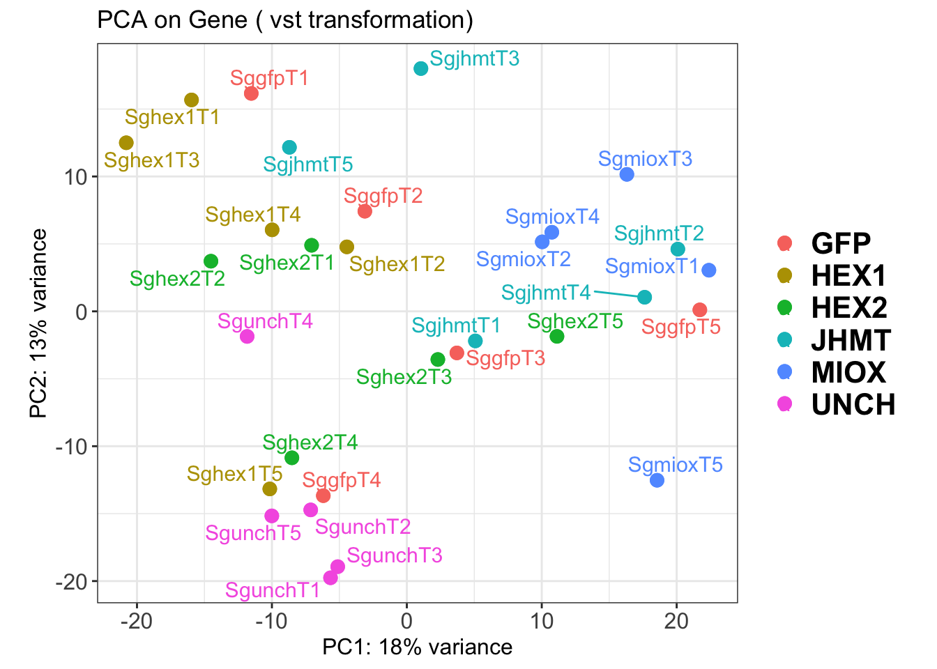
pca_results$PCA_Hull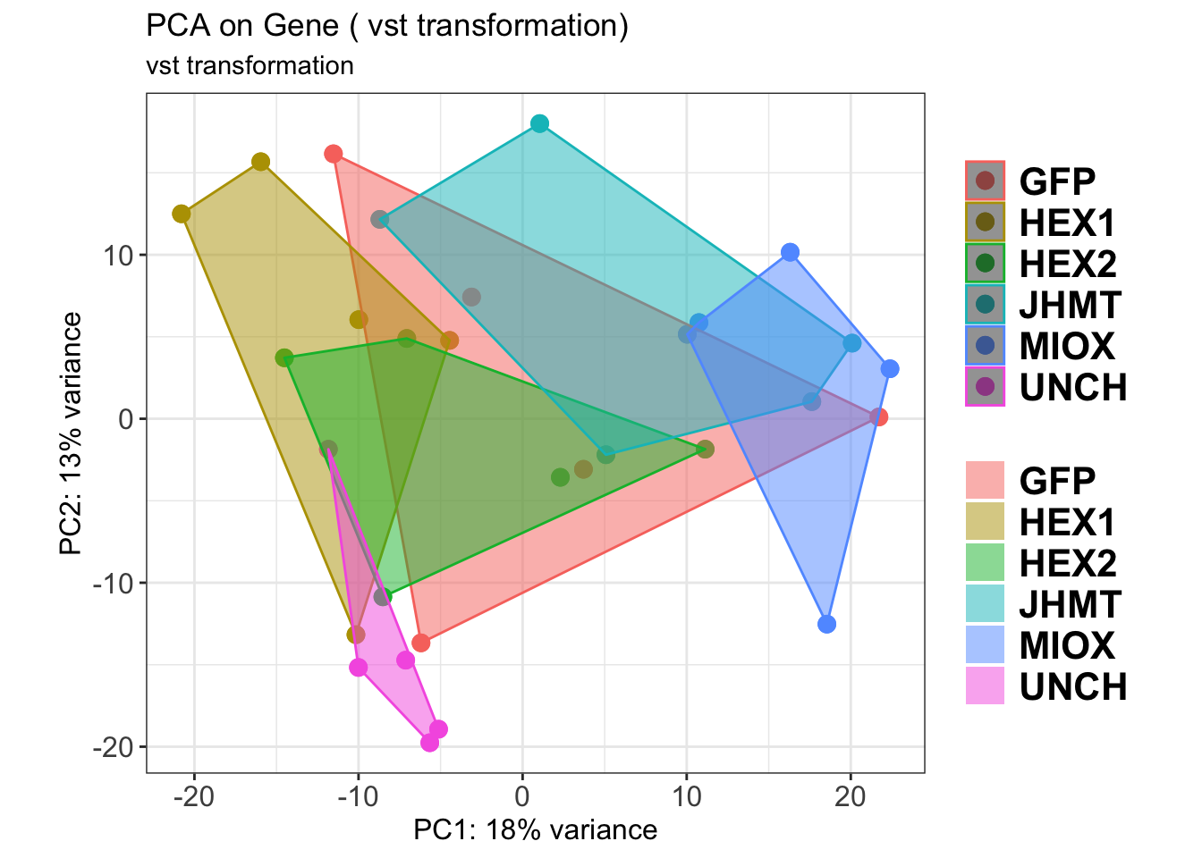
SVA
### SVA analysis to control for technical variation
dat <- counts(dds, normalized = TRUE)
idx <- rowMeans(dat) > 1
dat <- dat[idx, ]
mod <- model.matrix(~ Gene, colData(dds))
mod0 <- model.matrix(~ 1, colData(dds))
svseq <- svaseq(dat, mod, mod0)Number of significant surrogate variables is: 4
Iteration (out of 5 ):1 2 3 4 5 sva_plots <- create_sva_plots(svseq, dds, saveDir, intgroup = c("Tissue", "Gene"))
# Show stripcharts in the report
sva_plots$Stripcharts[[1]] # Show first stripchart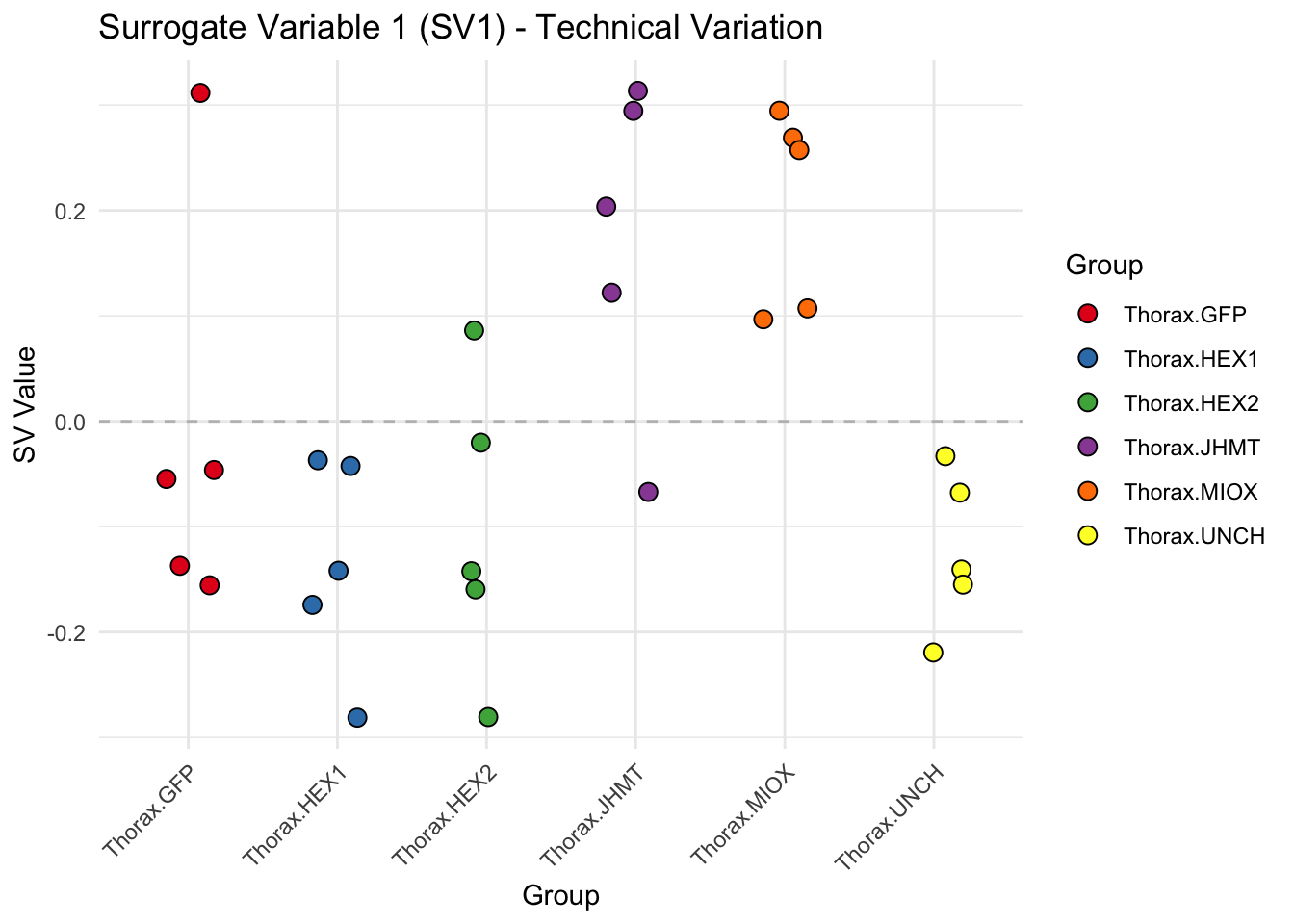
sva_plots$Stripcharts[[2]] # Show second stripchart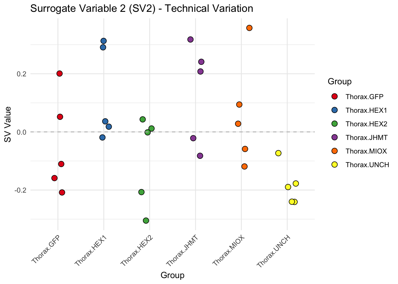
sva_plots$Stripcharts[[3]] # Show third stripchart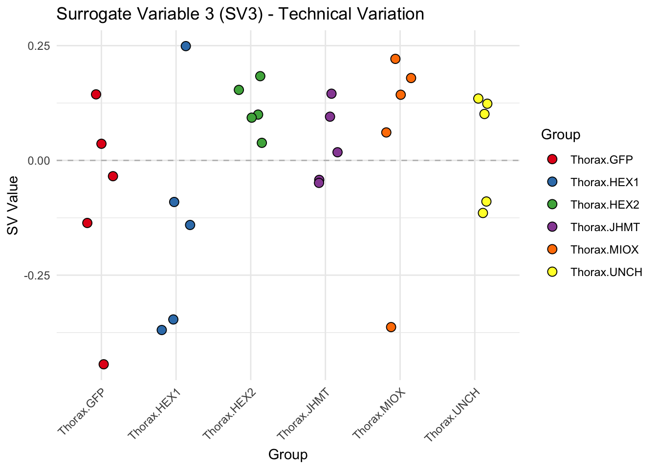
| Version | Author | Date |
|---|---|---|
| d7fa779 | Maeva TECHER | 2025-02-14 |
# Show scatter plots in the report
sva_plots$ScatterPlots[["1_2"]] # Show SV1 vs SV2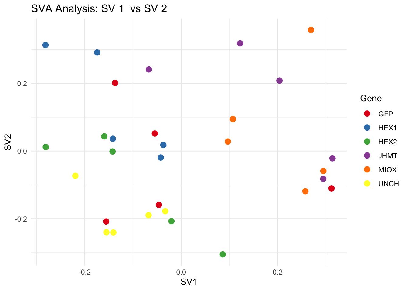
| Version | Author | Date |
|---|---|---|
| d7fa779 | Maeva TECHER | 2025-02-14 |
sva_plots$ScatterPlots[["1_3"]] # Show SV1 vs SV3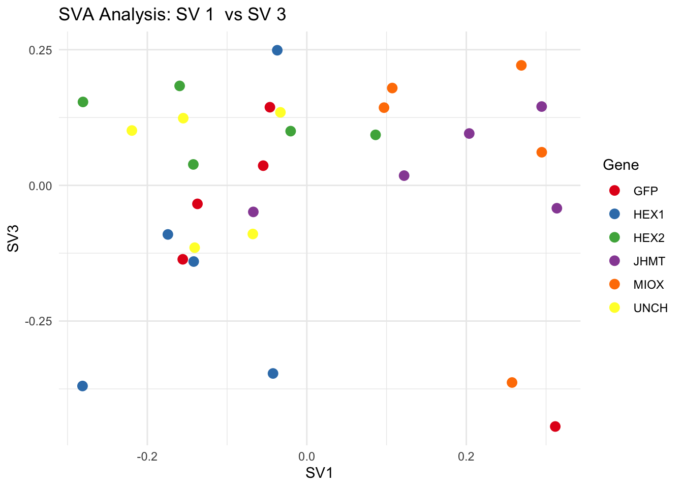
| Version | Author | Date |
|---|---|---|
| d7fa779 | Maeva TECHER | 2025-02-14 |
sva_plots$ScatterPlots[["2_3"]] # Show SV2 vs SV3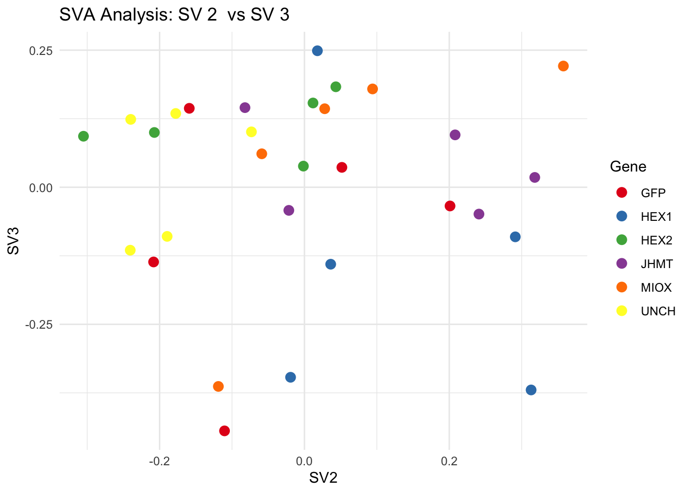
| Version | Author | Date |
|---|---|---|
| d7fa779 | Maeva TECHER | 2025-02-14 |
We rerun the DESeq2 model but this time including the
surrogate variable as a covariate, as we know that the modeled variation
is more likely explained by tissue and gene variation rather than batch
effects.
ddssva <- dds
ddssva$SV1 <- svseq$sv[,1]
ddssva$SV2 <- svseq$sv[,2]
ddssva$SV3 <- svseq$sv[,3]
design(ddssva) <- ~ SV1 + SV2 + SV3 + Gene
ddssva$Gene <- relevel(ddssva$Gene, ref = "GFP")
smallestGroupSize <- 5
keep <- rowSums(counts(ddssva) >= 10) >= smallestGroupSize
ddssva <- ddssva[keep,]
ddssva <- DESeq(ddssva)
ddssva <- ddssva[which(mcols(ddssva)$betaConv),] # remove non converging rows
### Extract results
message("Available contrasts are: ", paste(resultsNames(ddssva), collapse = ", "))
hex1 <- results(ddssva, name = "Gene_HEX1_vs_GFP", alpha = 0.05)
hex2 <- results(ddssva, name = "Gene_HEX2_vs_GFP", alpha = 0.05)
jhmt <- results(ddssva, name = "Gene_JHMT_vs_GFP", alpha = 0.05)
miox <- results(ddssva, name = "Gene_MIOX_vs_GFP", alpha = 0.05)
unch <- results(ddssva, name = "Gene_UNCH_vs_GFP", alpha = 0.05)Volcano plots and Heatmaps
First we create function to generate the plots we are interested to obtain and then run the whole pipeline for each gene.
# Define contrast_sets
hex1_samples <- c("SggfpT1","SggfpT2","SggfpT3","SggfpT4","SggfpT5",
"Sghex1T1","Sghex1T2","Sghex1T3","Sghex1T4","Sghex1T5")
hex2_samples <- c("SggfpT1","SggfpT2","SggfpT3","SggfpT4","SggfpT5",
"Sghex2T1","Sghex2T2","Sghex2T3","Sghex2T4","Sghex2T5")
jhmt_samples <- c("SggfpT1","SggfpT2","SggfpT3","SggfpT4","SggfpT5",
"SgjhmtT1","SgjhmtT2","SgjhmtT3","SgjhmtT4","SgjhmtT5")
miox_samples <- c("SggfpT1","SggfpT2","SggfpT3","SggfpT4","SggfpT5",
"SgmioxT1","SgmioxT2","SgmioxT3","SgmioxT4","SgmioxT5")
unch_samples <- c("SggfpT1","SggfpT2","SggfpT3","SggfpT4","SggfpT5",
"SgunchT1","SgunchT2","SgunchT3","SgunchT4","SgunchT5")
# Run full analysis
hex1_plots <- visualize_data(hex1, "HEX1_vs_GFP", hex1_samples)
hex2_plots <- visualize_data(hex2, "HEX2_vs_GFP", hex2_samples)
jhmt_plots <- visualize_data(jhmt, "JHMT_vs_GFP", jhmt_samples)
miox_plots <- visualize_data(miox, "MIOX_vs_GFP", miox_samples)
unch_plots <- visualize_data(unch, "UNCH_vs_GFP", unch_samples)
hex1_plots$volcano; hex1_plots$heatmap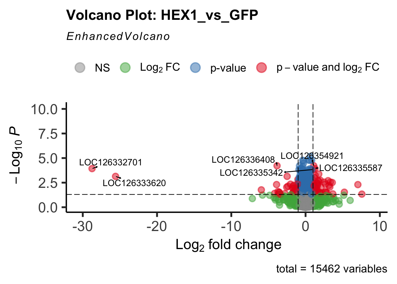
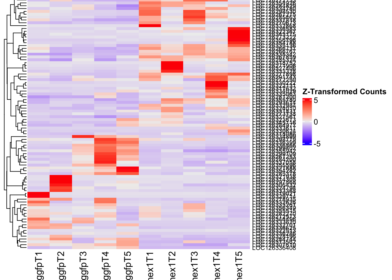
hex2_plots$volcano; hex2_plots$heatmap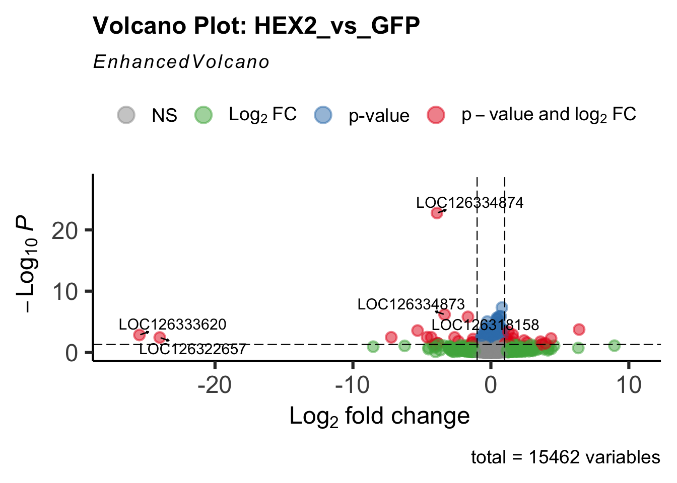
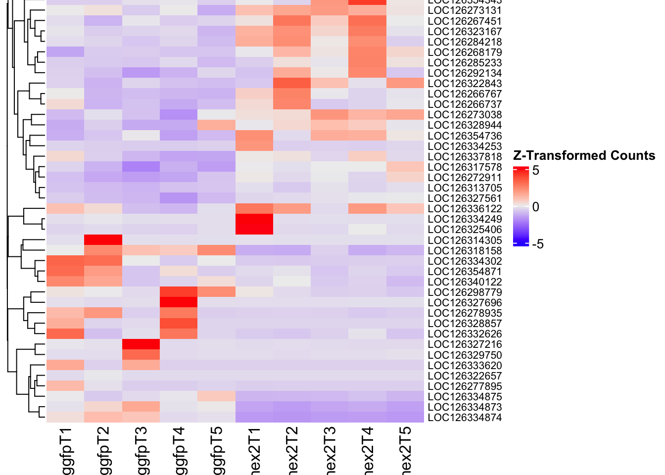
jhmt_plots$volcano; jhmt_plots$heatmap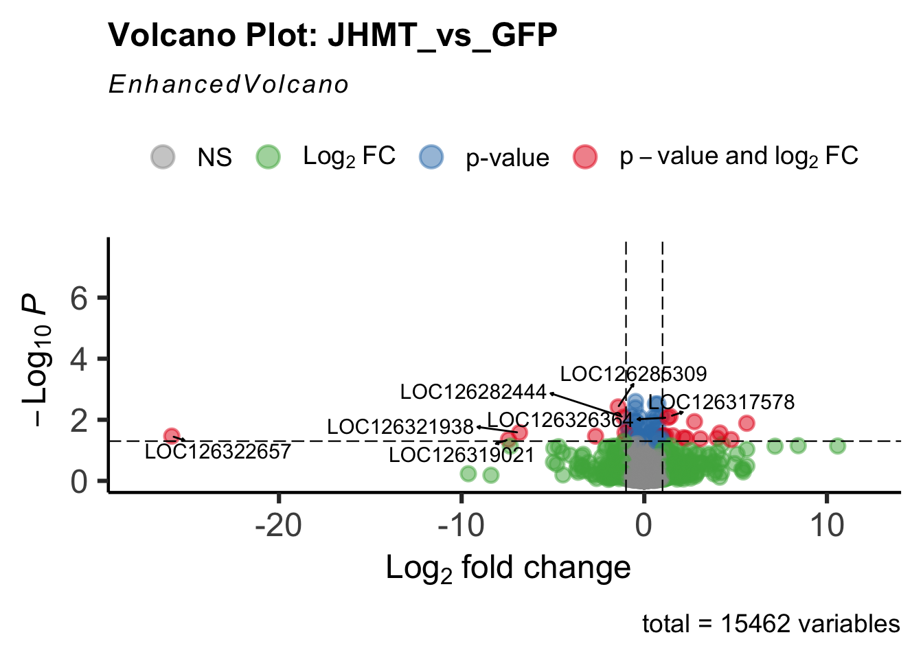
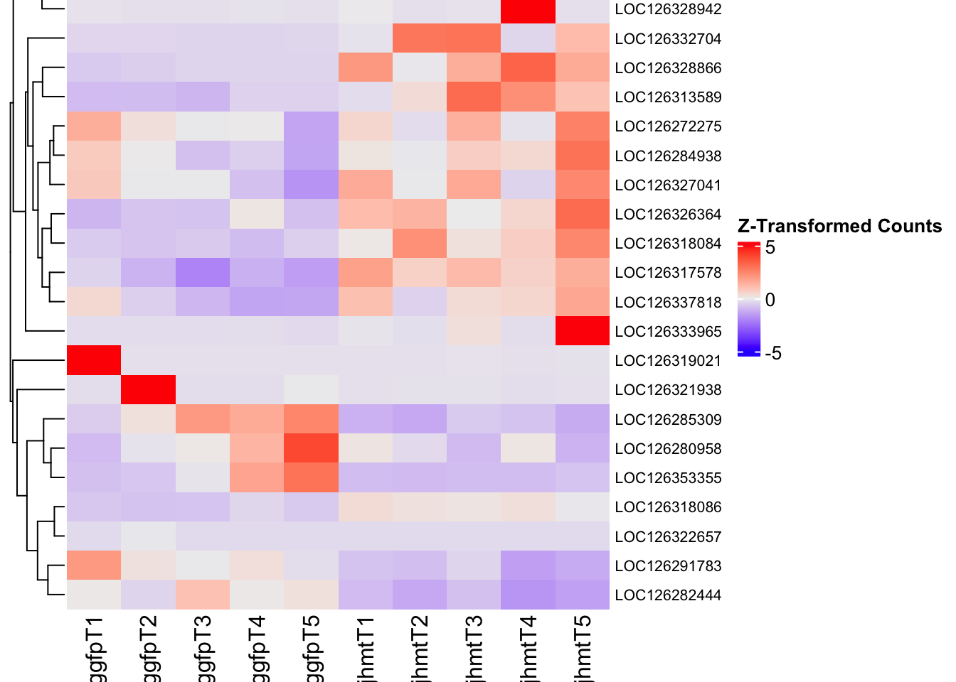
miox_plots$volcano; miox_plots$heatmap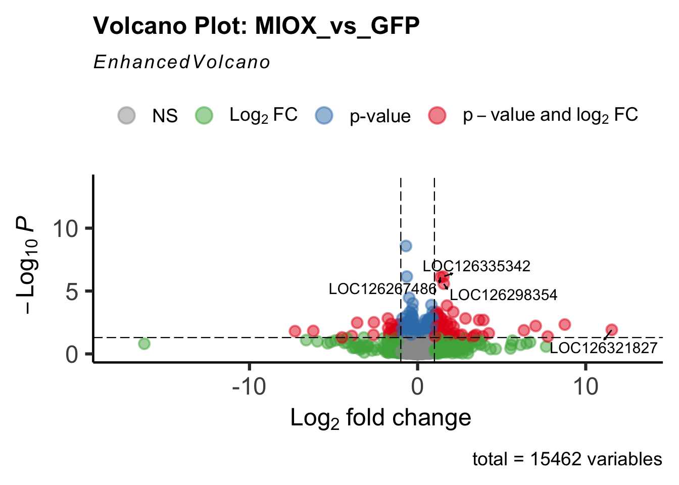
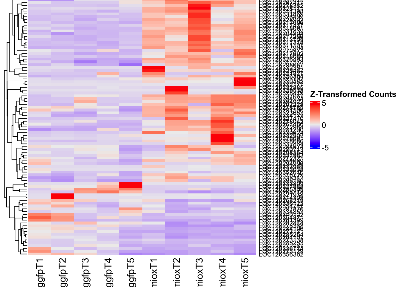
unch_plots$volcano; unch_plots$heatmap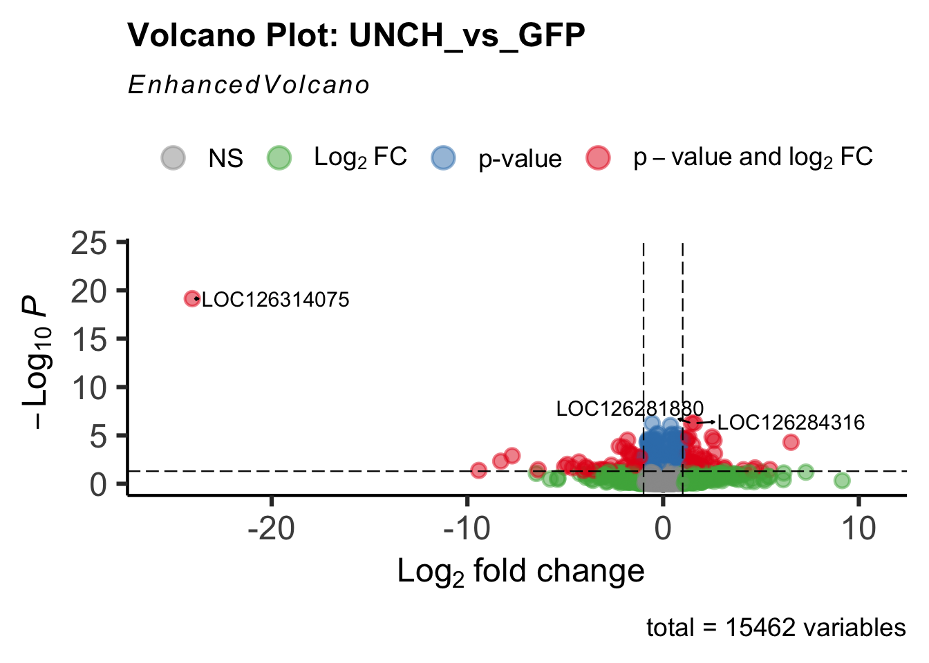
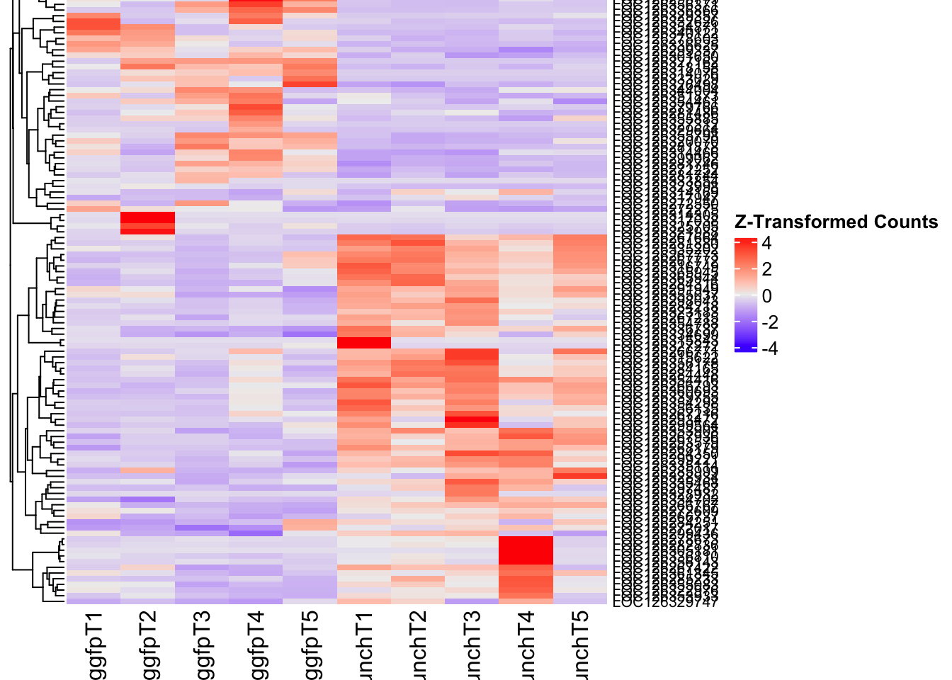
DEG tables
The following tables show the genes differentially expressed with at least an absolute log2fold change of > 1 considering thorax tissue only. Considering GFP as the reference state, upregulated genes in knockdown treatment in red and downregulated genes in knockdown treatment in blue. You can search for a gene of interest by writting a LOCID or description in the search bar or sort by column.
# Generate tables for each contrast
table_hex1 <- generate_deg_table(ddssva, "Gene_HEX1_vs_GFP", allspecies_df)
out of 15462 with nonzero total read count
adjusted p-value < 0.05
LFC > 0 (up) : 436, 2.8%
LFC < 0 (down) : 598, 3.9%
outliers [1] : 0, 0%
low counts [2] : 2998, 19%
(mean count < 27)
[1] see 'cooksCutoff' argument of ?results
[2] see 'independentFiltering' argument of ?resultsTotal DEGs p-value < 0.05 and absolute logFoldChange > 1: 93LFC > 1 (up) : 54 (58.06%)LFC < -1 (down) : 39 (41.94%)table_hex1$kable_tabletable_hex2 <- generate_deg_table(ddssva, "Gene_HEX2_vs_GFP", allspecies_df)
out of 15462 with nonzero total read count
adjusted p-value < 0.05
LFC > 0 (up) : 224, 1.4%
LFC < 0 (down) : 149, 0.96%
outliers [1] : 0, 0%
low counts [2] : 2399, 16%
(mean count < 21)
[1] see 'cooksCutoff' argument of ?results
[2] see 'independentFiltering' argument of ?resultsTotal DEGs p-value < 0.05 and absolute logFoldChange > 1: 43LFC > 1 (up) : 25 (58.14%)LFC < -1 (down) : 18 (41.86%)table_hex2$kable_tabletable_jhmt <- generate_deg_table(ddssva, "Gene_JHMT_vs_GFP", allspecies_df)
out of 15462 with nonzero total read count
adjusted p-value < 0.05
LFC > 0 (up) : 40, 0.26%
LFC < 0 (down) : 40, 0.26%
outliers [1] : 0, 0%
low counts [2] : 3298, 21%
(mean count < 31)
[1] see 'cooksCutoff' argument of ?results
[2] see 'independentFiltering' argument of ?resultsTotal DEGs p-value < 0.05 and absolute logFoldChange > 1: 22LFC > 1 (up) : 14 (63.64%)LFC < -1 (down) : 8 (36.36%)table_jhmt$kable_tabletable_miox <- generate_deg_table(ddssva, "Gene_MIOX_vs_GFP", allspecies_df)
out of 15462 with nonzero total read count
adjusted p-value < 0.05
LFC > 0 (up) : 226, 1.5%
LFC < 0 (down) : 230, 1.5%
outliers [1] : 0, 0%
low counts [2] : 2998, 19%
(mean count < 27)
[1] see 'cooksCutoff' argument of ?results
[2] see 'independentFiltering' argument of ?resultsTotal DEGs p-value < 0.05 and absolute logFoldChange > 1: 96LFC > 1 (up) : 69 (71.88%)LFC < -1 (down) : 27 (28.12%)table_miox$kable_tabletable_unch <- generate_deg_table(ddssva, "Gene_UNCH_vs_GFP", allspecies_df)
out of 15462 with nonzero total read count
adjusted p-value < 0.05
LFC > 0 (up) : 256, 1.7%
LFC < 0 (down) : 251, 1.6%
outliers [1] : 0, 0%
low counts [2] : 1499, 9.7%
(mean count < 13)
[1] see 'cooksCutoff' argument of ?results
[2] see 'independentFiltering' argument of ?resultsTotal DEGs p-value < 0.05 and absolute logFoldChange > 1: 113LFC > 1 (up) : 67 (59.29%)LFC < -1 (down) : 46 (40.71%)table_unch$kable_tableSummary and Overlap
# Summarize DEGs for all contrasts
deg_summary <- bind_rows(
summarize_deg_counts(table_hex1, "HEX1 vs GFP"),
summarize_deg_counts(table_hex2, "HEX2 vs GFP"),
summarize_deg_counts(table_jhmt, "JHMT vs GFP"),
summarize_deg_counts(table_miox, "MIOX vs GFP"),
summarize_deg_counts(table_unch, "UNCH vs GFP")
)
# Display table using kable with styling
deg_summary %>%
kable("html", escape = FALSE, col.names = gsub("_", " ", names(.))) %>%
kable_styling("striped", full_width = TRUE) %>%
column_spec(2, color = "red", bold = TRUE) %>% # Upregulated in red
column_spec(3, color = "blue", bold = TRUE) %>% # Downregulated in blue
add_header_above(c("Summary of DEGs" = 3)) %>%
row_spec(0, bold = TRUE)| Contrast | Upregulated | Downregulated |
|---|---|---|
| HEX1 vs GFP | 50 | 36 |
| HEX2 vs GFP | 20 | 17 |
| JHMT vs GFP | 14 | 8 |
| MIOX vs GFP | 65 | 24 |
| UNCH vs GFP | 63 | 43 |
# Define the list of RNAi contrasts
contrast_list <- c("HEX1_vs_GFP", "HEX2_vs_GFP", "JHMT_vs_GFP",
"MIOX_vs_GFP", "UNCH_vs_GFP")
# Initialize empty lists for storing Head-specific DEGs for each contrast
venn_data_up <- list()
venn_data_down <- list()
venn_data_all <- list()
# Function to load Head-specific DEGs for a given set of contrasts
load_deg_contrasts_head <- function(contrast_list) {
degs_up <- list()
degs_down <- list()
degs_all <- list()
for (contrast in contrast_list) {
deg_file <- file.path(workDir, "DEG_results/RNAi/Thorax/", contrast, paste0("DEG_sigresults_", contrast, ".csv"))
if (!file.exists(deg_file)) {
message(paste("File missing for contrast:", contrast))
next # Skip if the file doesn't exist
}
deg_data <- read.csv(deg_file, stringsAsFactors = FALSE)
# Convert row names to a column if necessary
if ("X" %in% colnames(deg_data)) {
colnames(deg_data)[colnames(deg_data) == "X"] <- "GeneID"
}
# Check if data is empty
if (nrow(deg_data) == 0) {
message(paste("No data for contrast:", contrast))
next
}
# Select significant DEGs (Up, Down, All)
degs_up[[contrast]] <- deg_data %>%
filter(padj < 0.05 & log2FoldChange >= 1) %>%
pull(GeneID) # Extract GeneID column
degs_down[[contrast]] <- deg_data %>%
filter(padj < 0.05 & log2FoldChange <= -1) %>%
pull(GeneID) # Extract GeneID column
degs_all[[contrast]] <- deg_data %>%
filter(padj < 0.05 & abs(log2FoldChange) >= 1) %>%
pull(GeneID) # Extract GeneID column
}
return(list(up = degs_up, down = degs_down, all = degs_all))
}
# Load DEG data for the defined contrasts (Head tissue only)
venn_data_contrasts <- load_deg_contrasts_head(contrast_list)
# Prepare the data for the Venn diagrams
venn_data_up <- venn_data_contrasts$up
venn_data_down <- venn_data_contrasts$down
venn_data_all <- venn_data_contrasts$all
# Function to display Venn diagram and corresponding datatable
display_venn_with_datatable <- function(venn_data, title, allspecies_df) {
# Calculate the overlapping genes
overlap_genes <- Reduce(intersect, venn_data)
# Create a data frame for the overlapping genes
overlap_df <- data.frame(GeneID = overlap_genes)
# Merge to get species information
meta_brock_df <- merge(overlap_df, allspecies_df, by = "GeneID", all.x = TRUE)
# Generate the Venn diagram
venn_plot <- venn.diagram(
x = venn_data,
category.names = contrast_list,
filename = NULL,
output = TRUE,
fill = c("orange", "red", "blue", "purple", "green"), # Adjust colors for contrasts
alpha = 0.5,
cex = 2,
cat.cex = 0,
main = title,
main.cex = 1.2
)
# Clear the plotting area before drawing
grid.newpage()
grid.draw(venn_plot)
# Create a custom legend
legend_labels <- contrast_list
legend_colors <- c("orange", "red", "blue", "purple", "green")
# Positioning the legend
legend_x <- unit(0.85, "npc") # Adjust x position
legend_y <- unit(0.2, "npc") # Adjust y position
# Draw the legend
for (i in 1:length(legend_labels)) {
grid.rect(x = legend_x, y = legend_y - unit((i - 1) * 0.05, "npc"),
width = unit(0.02, "npc"), height = unit(0.02, "npc"),
gp = gpar(fill = legend_colors[i], col = NA))
grid.text(label = legend_labels[i], x = legend_x + unit(0.05, "npc"),
y = legend_y - unit((i - 1) * 0.05, "npc"),
just = "left", gp = gpar(cex = 0.8))
}
# Display the merged overlapping genes table with datatable
datatable(meta_brock_df, options = list(
pageLength = 10,
scrollX = TRUE,
autoWidth = TRUE,
searchHighlight = TRUE
),
rownames = FALSE,
escape = FALSE
) %>%
formatStyle(
'Species', target = 'cell',
fontStyle = 'italic'
) %>%
formatStyle(
columns = names(meta_brock_df),
target = 'row',
color = styleEqual(c("red", "blue", "black"), c("red", "blue", "black")),
fontWeight = styleEqual(c("bold", "normal"), c("bold", "normal")),
backgroundColor = styleEqual(c("red", "blue", "black"), c("white", "white", "white"))
)
}
# Display the Venn diagram and datatable for **Head Upregulated DEGs** across contrasts
display_venn_with_datatable(venn_data_up, "Venn Diagram of Head Upregulated DEGs - RNAi Contrasts", allspecies_df)
| Version | Author | Date |
|---|---|---|
| b540a1e | Maeva TECHER | 2025-02-27 |
# Display the Venn diagram and datatable for **Head Downregulated DEGs** across contrasts
display_venn_with_datatable(venn_data_down, "Venn Diagram of Head Downregulated DEGs - RNAi Contrasts", allspecies_df)
# Display the Venn diagram and datatable for **All Significant DEGs in Head Tissue**
display_venn_with_datatable(venn_data_all, "Venn Diagram of All Significant DEGs in Head Tissue - RNAi Contrasts", allspecies_df)
| Version | Author | Date |
|---|---|---|
| b540a1e | Maeva TECHER | 2025-02-27 |
GO and KEGG enrichment
#enrich_data(hex1, "Hex1_vs_GFP", hex1_samples)
#enrich_data(hex2, "Hex2_vs_GFP", hex2_samples)
#enrich_data(jhmt, "JHMT_vs_GFP", jhmt_samples)
#enrich_data(miox, "MIOX_vs_GFP", miox_samples)
#enrich_data(unch, "UNCH_vs_GFP", unch_samples)Excluding rRNA
All tissue together
Minor changes here are made compared to the DESeq2
results regarding the importation of samples to transform into a
matrix.
Sample names are structured as follow: {Sg}{gene}{#} {Sg} = Schistocerca gregaria {gene} = gene abbreviation gfp, hex1, hex2, jhmt, miox and unch H/T{#} = biological replicate
saveDir <- paste0(workDir,"/DEG_results/RNAi/All_no_rRNA")
dir.create(saveDir)
### Prepare Sample CSV file #####
samples <- read.delim(file.path(workDir, "list/RNAi/All_RNAisample_list.csv"), sep = ",", row.names = 1, header = TRUE)
files <- file.path(workDir, "readcounts/RNAi/", samples$Tissue, samples$Filename)
names(files) <- row.names(samples)
if (all(file.exists(files))) {
message("All the files exist!")
} else {
warning("Some files are missing!")
}All the files exist!### Create count sample matrix
cts <- map_dfc(files, function(sample) {
data_count <- read.delim(sample, sep = "\t", header = FALSE)
col_name <- gsub("_counts.txt", "", basename(sample))
setNames(data.frame(data_count[, 2]), col_name)
})
row_get <- read.delim(files[1], sep = "\t", row.names = 1, header = F) # Get proper row names
rownames(cts) <- rownames(row_get)
rm(row_get) # remove unused object from memoryWhile for bulk RNAseq on head and thorax for all species, the DEGs model was made between isolated and crowded individuals (with isolated as the reference state), here, the DEG analysis will be carried between GFP knock-down nymphs (as reference state) vs Hexamerins / Juvenile Hormones / Inositol / Uncharacterized proteins.
### Build DESeq2 Object
dds <- DESeqDataSetFromMatrix(countData = cts,
colData = samples,
design = ~ Gene)
dds$Gene <- relevel(dds$Gene, ref = "GFP")
smallestGroupSize <- 5
keep <- rowSums(counts(dds) >= 10) >= smallestGroupSize
dds <- dds[keep,]
loci_to_exclude <- readLines(file.path(workDir, "list/excluded_loci/gregaria_rrna_list.txt"))
dds <- dds[!(rownames(dds) %in% loci_to_exclude), ]
dds <- DESeq(dds)Normalization and PCA
# Plot PCA and investigate quality metrics
vsd <- vst(dds, blind = TRUE)
# Perform PCA
pca_data <- plotPCA(vsd, intgroup = c("Tissue", "Gene"), returnData = TRUE)
# Define colors for genes (slightly transparent) and shapes for tissues
gene_colors <- scale_color_manual(values = alpha(brewer.pal(n = length(unique(pca_data$Gene)), name = "Set1"), 0.8)) # Points are transparent
tissue_shapes <- scale_shape_manual(values = seq(15, 15 + length(unique(pca_data$Tissue))))
# **PCA without labels**
p_pca_nolabel <- ggplot(pca_data, aes(x = PC1, y = PC2, color = Gene, shape = Tissue)) +
geom_point(size = 4) +
gene_colors +
tissue_shapes +
theme_bw() +
theme(legend.title = element_blank(),
legend.text = element_text(face = "bold", size = 14),
axis.text = element_text(size = 12),
axis.title = element_text(size = 14)) +
ggtitle("PCA of All Tissues (No Labels)", subtitle = "Tissues differentiated by shape, Genes by color")
# Save PCA without labels
ggsave(paste0(saveDir, "/PCA_Tissue_Gene_NoLabel.png"), plot = p_pca_nolabel, width = 10, height = 10, dpi = 600, device = "png")
# **PCA with labels**
p_pca_label <- ggplot(pca_data, aes(x = PC1, y = PC2, color = Gene, shape = Tissue)) +
geom_point(size = 4) +
geom_text_repel(aes(label = name), size = 4, color = "black", max.overlaps = 20) + # Labels are fully visible
gene_colors +
tissue_shapes +
theme_bw() +
theme(legend.title = element_blank(),
legend.text = element_text(face = "bold", size = 14),
axis.text = element_text(size = 12),
axis.title = element_text(size = 14)) +
ggtitle("PCA of All Tissues (With Labels)", subtitle = "Tissues differentiated by shape, Genes by color")
# Save PCA with labels
ggsave(paste0(saveDir, "/PCA_Tissue_Gene_Label.png"), plot = p_pca_label, width = 10, height = 10, dpi = 600, device = "png")
# **Return plots for knitr/RMarkdown**
list(NoLabel = p_pca_nolabel, WithLabel = p_pca_label)$NoLabel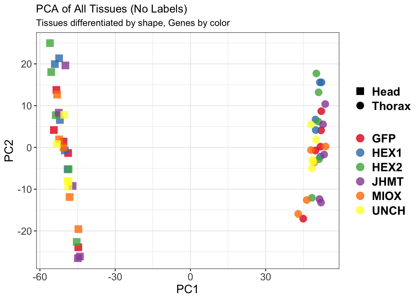
| Version | Author | Date |
|---|---|---|
| d7fa779 | Maeva TECHER | 2025-02-14 |
$WithLabel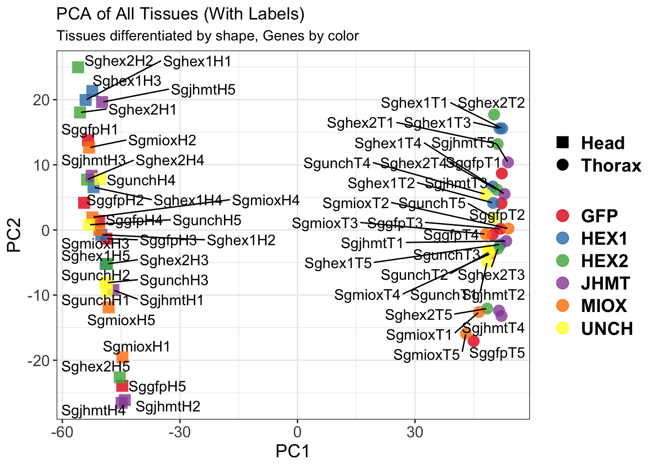
| Version | Author | Date |
|---|---|---|
| d7fa779 | Maeva TECHER | 2025-02-14 |
The PCA plot shows clear distinction between tissue types, while gene silencing has a large variation within each tissue, and presents no distinct clear groupings for a single gene.
SVA
### SVA analysis to control for technical variation
dat <- counts(dds, normalized = TRUE)
idx <- rowMeans(dat) > 1
dat <- dat[idx, ]
mod <- model.matrix(~ Gene, colData(dds))
mod0 <- model.matrix(~ 1, colData(dds))
svseq <- svaseq(dat, mod, mod0)Number of significant surrogate variables is: 2
Iteration (out of 5 ):1 2 3 4 5 sva_plots <- create_sva_plots(svseq, dds, saveDir, intgroup = c("Tissue", "Gene"), max_sv = 5)
# Show stripcharts in the report
sva_plots$Stripcharts[[1]] # Show first stripchart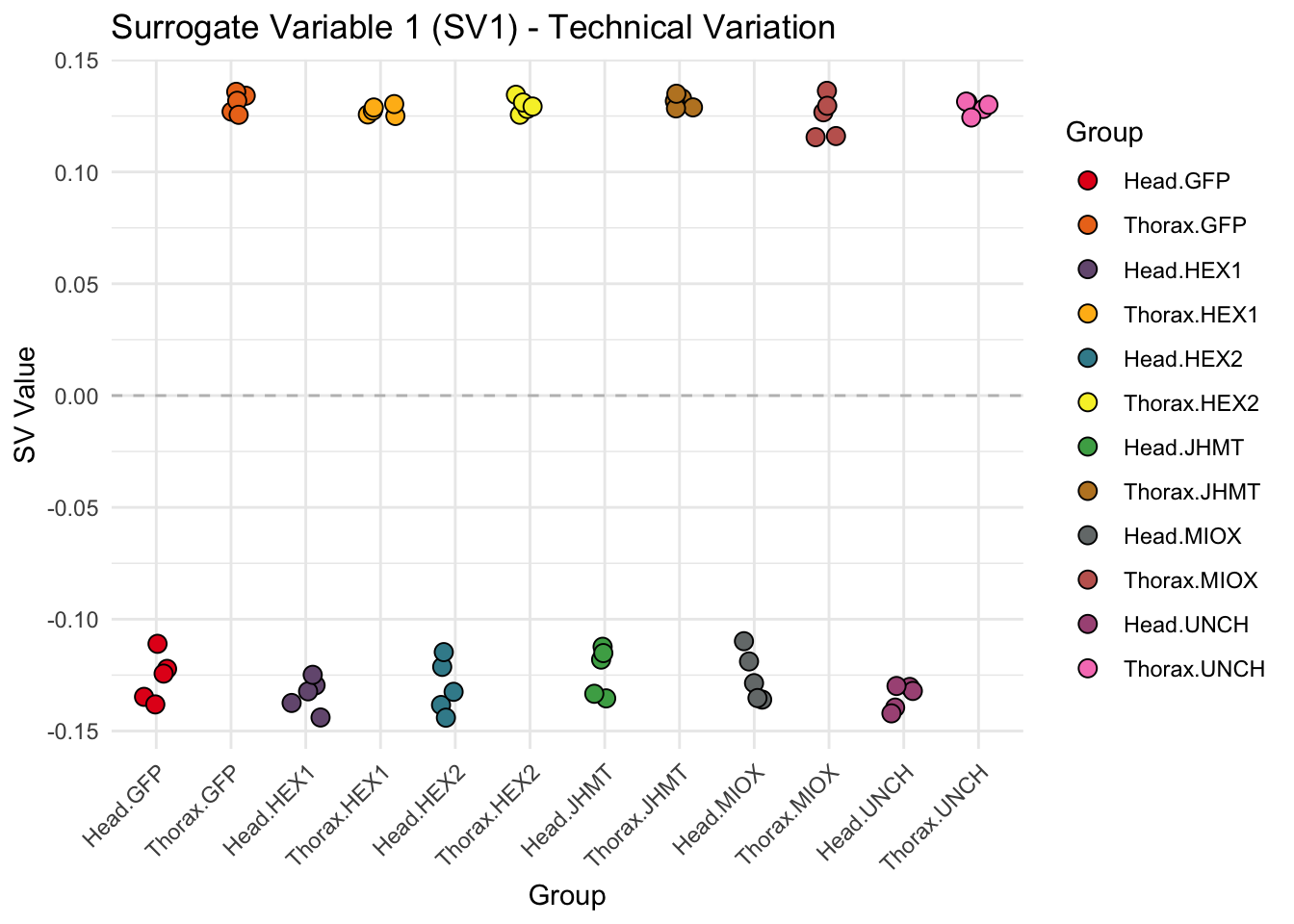
sva_plots$Stripcharts[[2]] # Show second stripchart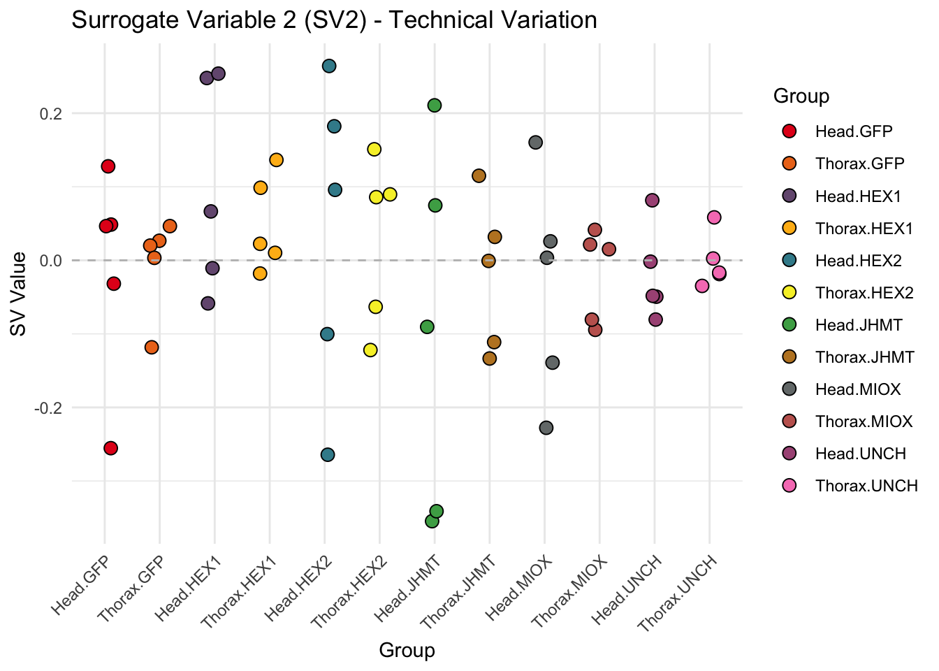
# Show scatter plots in the report
sva_plots$ScatterPlots[["1_2"]] # Show SV1 vs SV2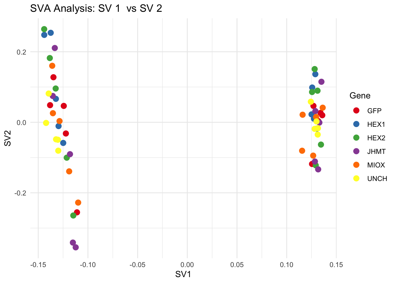
SV1 is clearly showing an effect of tissue. We rerun the
DESeq2 model but this time including the surrogate variable
SV2 and SV3 as a covariates only, as we know that the modeled variation
is more likely explained by tissue and gene variation rather than batch
effects.
ddssva <- dds
ddssva$SV1 <- svseq$sv[,1]
ddssva$SV2 <- svseq$sv[,2]
design(ddssva) <- ~ SV2 + Gene
ddssva$Gene <- relevel(ddssva$Gene, ref = "GFP")
smallestGroupSize <- 5
keep <- rowSums(counts(ddssva) >= 10) >= smallestGroupSize
ddssva <- ddssva[keep,]
ddssva <- DESeq(ddssva)
ddssva <- ddssva[which(mcols(ddssva)$betaConv),] # remove non converging rows
### Extract results
message("Available contrasts are: ", paste(resultsNames(ddssva), collapse = ", "))
hex1 <- results(ddssva, name = "Gene_HEX1_vs_GFP", alpha = 0.05)
hex2 <- results(ddssva, name = "Gene_HEX2_vs_GFP", alpha = 0.05)
jhmt <- results(ddssva, name = "Gene_JHMT_vs_GFP", alpha = 0.05)
miox <- results(ddssva, name = "Gene_MIOX_vs_GFP", alpha = 0.05)
unch <- results(ddssva, name = "Gene_UNCH_vs_GFP", alpha = 0.05)Volcano plots and Heatmaps
# Define contrast_sets
hex1_samples <- c("SggfpH1","SggfpH2","SggfpH3","SggfpH4","SggfpH5",
"Sghex1H1","Sghex1H2","Sghex1H3","Sghex1H4","Sghex1H5",
"SggfpT1","SggfpT2","SggfpT3","SggfpT4","SggfpT5",
"Sghex1T1","Sghex1T2","Sghex1T3","Sghex1T4","Sghex1T5")
hex2_samples <- c("SggfpH1","SggfpH2","SggfpH3","SggfpH4","SggfpH5",
"Sghex2H1","Sghex2H2","Sghex2H3","Sghex2H4","Sghex2H5",
"SggfpT1","SggfpT2","SggfpT3","SggfpT4","SggfpT5",
"Sghex2T1","Sghex2T2","Sghex2T3","Sghex2T4","Sghex2T5")
jhmt_samples <- c("SggfpH1","SggfpH2","SggfpH3","SggfpH4","SggfpH5",
"SgjhmtH1","SgjhmtH2","SgjhmtH3","SgjhmtH4","SgjhmtH5",
"SggfpT1","SggfpT2","SggfpT3","SggfpT4","SggfpT5",
"SgjhmtT1","SgjhmtT2","SgjhmtT3","SgjhmtT4","SgjhmtT5")
miox_samples <- c("SggfpH1","SggfpH2","SggfpH3","SggfpH4","SggfpH5",
"SgmioxH1","SgmioxH2","SgmioxH3","SgmioxH4","SgmioxH5",
"SggfpT1","SggfpT2","SggfpT3","SggfpT4","SggfpT5",
"SgmioxT1","SgmioxT2","SgmioxT3","SgmioxT4","SgmioxT5")
unch_samples <- c("SggfpH1","SggfpH2","SggfpH3","SggfpH4","SggfpH5",
"SgunchH1","SgunchH2","SgunchH3","SgunchH4","SgunchH5",
"SggfpT1","SggfpT2","SggfpT3","SggfpT4","SggfpT5",
"SgunchT1","SgunchT2","SgunchT3","SgunchT4","SgunchT5")
# Run full analysis
hex1_plots <- visualize_data(hex1, "HEX1_vs_GFP", hex1_samples)
hex2_plots <- visualize_data(hex2, "HEX2_vs_GFP", hex2_samples)
jhmt_plots <- visualize_data(jhmt, "JHMT_vs_GFP", jhmt_samples)
miox_plots <- visualize_data(miox, "MIOX_vs_GFP", miox_samples)
unch_plots <- visualize_data(unch, "UNCH_vs_GFP", unch_samples)
hex1_plots$volcano; hex1_plots$heatmap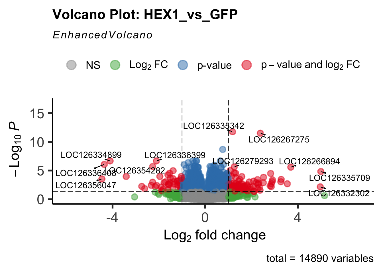
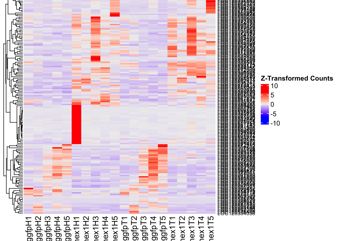
hex2_plots$volcano; hex2_plots$heatmap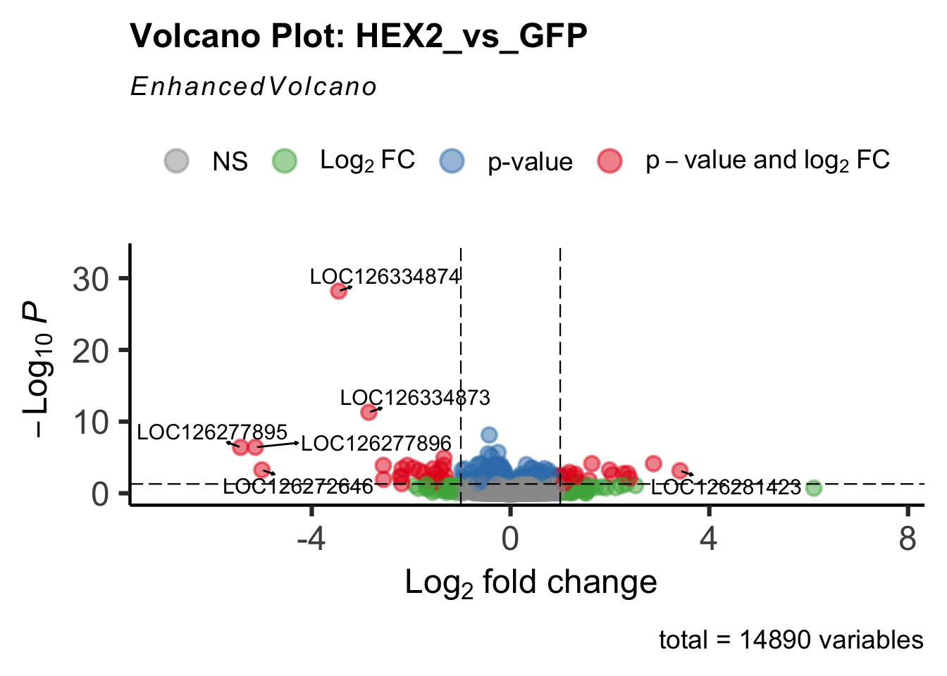
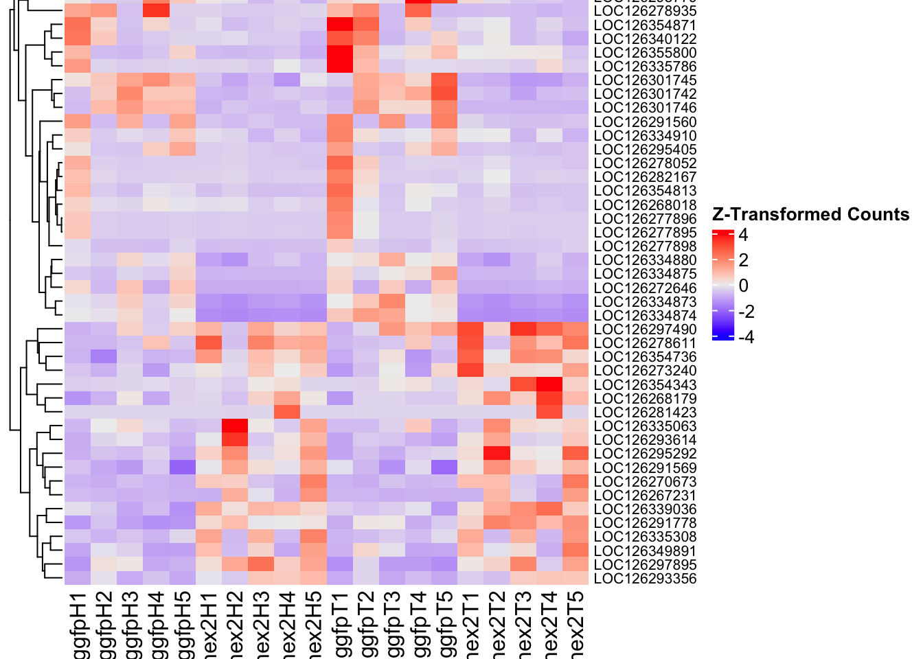
jhmt_plots$volcano; jhmt_plots$heatmap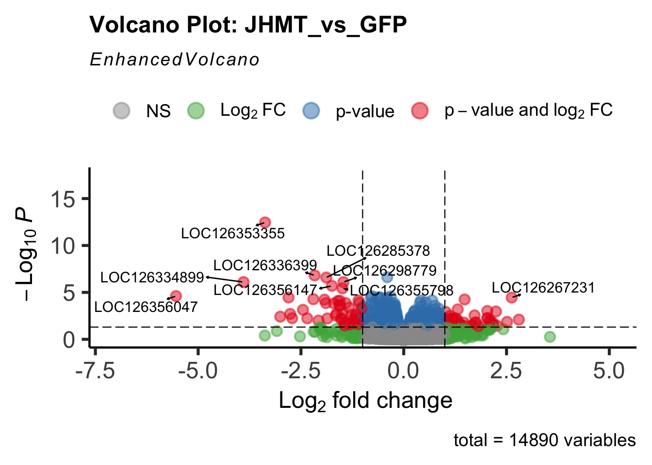
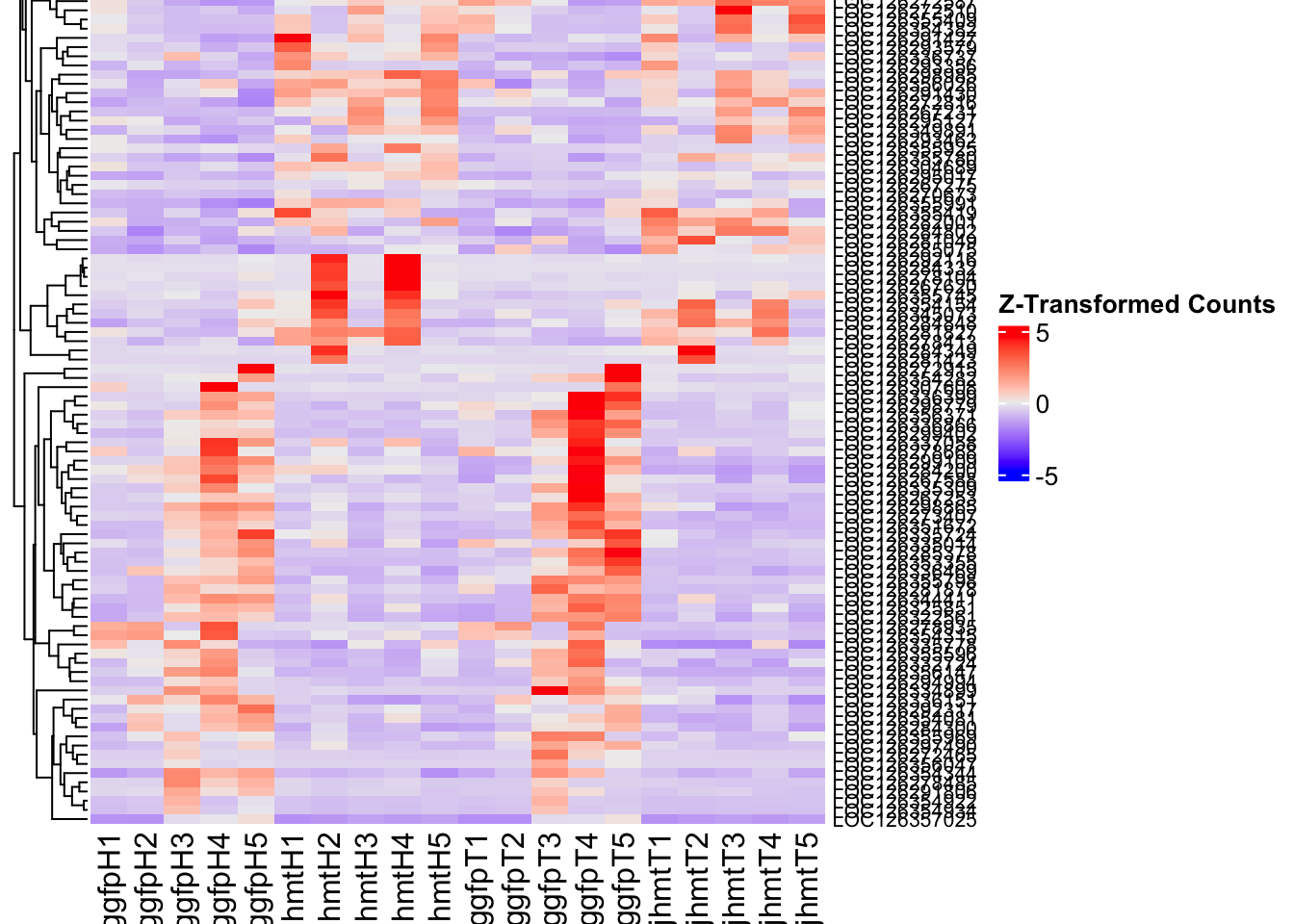
miox_plots$volcano; miox_plots$heatmap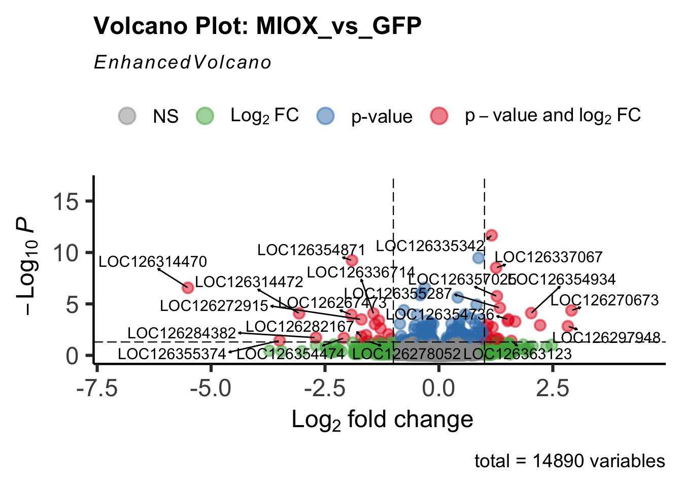
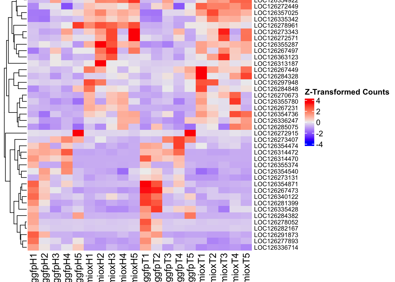
unch_plots$volcano; unch_plots$heatmap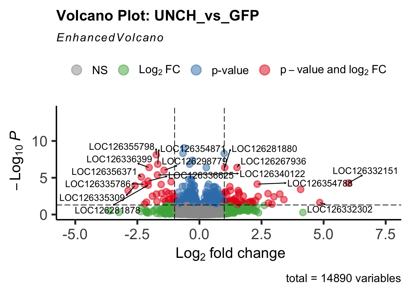
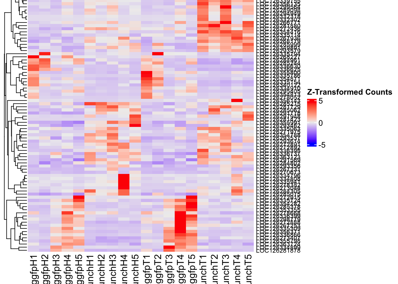
DEG tables
The following tables show the genes differentially expressed with at least an absolute log2fold change of > 1 considering all tissues together. Considering GFP as the reference state, upregulated genes in knockdown treatment in red and downregulated genes in knockdown treatment in blue. You can search for a gene of interest by writting a LOCID or description in the search bar or sort by column.
# Generate tables for each contrast
table_hex1 <- generate_deg_table(ddssva, "Gene_HEX1_vs_GFP", allspecies_df)
out of 14890 with nonzero total read count
adjusted p-value < 0.05
LFC > 0 (up) : 839, 5.6%
LFC < 0 (down) : 950, 6.4%
outliers [1] : 0, 0%
low counts [2] : 0, 0%
(mean count < 2)
[1] see 'cooksCutoff' argument of ?results
[2] see 'independentFiltering' argument of ?resultsTotal DEGs p-value < 0.05 and absolute logFoldChange > 1: 157LFC > 1 (up) : 110 (70.06%)LFC < -1 (down) : 47 (29.94%)table_hex1$kable_tabletable_hex2 <- generate_deg_table(ddssva, "Gene_HEX2_vs_GFP", allspecies_df)
out of 14890 with nonzero total read count
adjusted p-value < 0.05
LFC > 0 (up) : 201, 1.3%
LFC < 0 (down) : 321, 2.2%
outliers [1] : 0, 0%
low counts [2] : 1444, 9.7%
(mean count < 13)
[1] see 'cooksCutoff' argument of ?results
[2] see 'independentFiltering' argument of ?resultsTotal DEGs p-value < 0.05 and absolute logFoldChange > 1: 45LFC > 1 (up) : 19 (42.22%)LFC < -1 (down) : 26 (57.78%)table_hex2$kable_tabletable_jhmt <- generate_deg_table(ddssva, "Gene_JHMT_vs_GFP", allspecies_df)
out of 14890 with nonzero total read count
adjusted p-value < 0.05
LFC > 0 (up) : 266, 1.8%
LFC < 0 (down) : 486, 3.3%
outliers [1] : 0, 0%
low counts [2] : 0, 0%
(mean count < 2)
[1] see 'cooksCutoff' argument of ?results
[2] see 'independentFiltering' argument of ?resultsTotal DEGs p-value < 0.05 and absolute logFoldChange > 1: 95LFC > 1 (up) : 44 (46.32%)LFC < -1 (down) : 51 (53.68%)table_jhmt$kable_tabletable_miox <- generate_deg_table(ddssva, "Gene_MIOX_vs_GFP", allspecies_df)
out of 14890 with nonzero total read count
adjusted p-value < 0.05
LFC > 0 (up) : 111, 0.75%
LFC < 0 (down) : 100, 0.67%
outliers [1] : 0, 0%
low counts [2] : 0, 0%
(mean count < 2)
[1] see 'cooksCutoff' argument of ?results
[2] see 'independentFiltering' argument of ?resultsTotal DEGs p-value < 0.05 and absolute logFoldChange > 1: 42LFC > 1 (up) : 23 (54.76%)LFC < -1 (down) : 19 (45.24%)table_miox$kable_tabletable_unch <- generate_deg_table(ddssva, "Gene_UNCH_vs_GFP", allspecies_df)
out of 14890 with nonzero total read count
adjusted p-value < 0.05
LFC > 0 (up) : 172, 1.2%
LFC < 0 (down) : 231, 1.6%
outliers [1] : 0, 0%
low counts [2] : 0, 0%
(mean count < 2)
[1] see 'cooksCutoff' argument of ?results
[2] see 'independentFiltering' argument of ?resultsTotal DEGs p-value < 0.05 and absolute logFoldChange > 1: 86LFC > 1 (up) : 53 (61.63%)LFC < -1 (down) : 33 (38.37%)table_unch$kable_tableSummary and Overlap
# Summarize DEGs for all contrasts
deg_summary <- bind_rows(
summarize_deg_counts(table_hex1, "HEX1 vs GFP"),
summarize_deg_counts(table_hex2, "HEX2 vs GFP"),
summarize_deg_counts(table_jhmt, "JHMT vs GFP"),
summarize_deg_counts(table_miox, "MIOX vs GFP"),
summarize_deg_counts(table_unch, "UNCH vs GFP")
)
# Display table using kable with styling
deg_summary %>%
kable("html", escape = FALSE, col.names = gsub("_", " ", names(.))) %>%
kable_styling("striped", full_width = TRUE) %>%
column_spec(2, color = "red", bold = TRUE) %>% # Upregulated in red
column_spec(3, color = "blue", bold = TRUE) %>% # Downregulated in blue
add_header_above(c("Summary of DEGs" = 3)) %>%
row_spec(0, bold = TRUE)| Contrast | Upregulated | Downregulated |
|---|---|---|
| HEX1 vs GFP | 107 | 45 |
| HEX2 vs GFP | 17 | 26 |
| JHMT vs GFP | 43 | 50 |
| MIOX vs GFP | 23 | 18 |
| UNCH vs GFP | 50 | 33 |
# Define the list of RNAi contrasts
contrast_list <- c("HEX1_vs_GFP", "HEX2_vs_GFP", "JHMT_vs_GFP",
"MIOX_vs_GFP", "UNCH_vs_GFP")
# Initialize empty lists for storing Head-specific DEGs for each contrast
venn_data_up <- list()
venn_data_down <- list()
venn_data_all <- list()
# Function to load Head-specific DEGs for a given set of contrasts
load_deg_contrasts_head <- function(contrast_list) {
degs_up <- list()
degs_down <- list()
degs_all <- list()
for (contrast in contrast_list) {
deg_file <- file.path(workDir, "DEG_results/RNAi/All_no_rRNA/", contrast, paste0("DEG_sigresults_", contrast, ".csv"))
if (!file.exists(deg_file)) {
message(paste("File missing for contrast:", contrast))
next # Skip if the file doesn't exist
}
deg_data <- read.csv(deg_file, stringsAsFactors = FALSE)
# Convert row names to a column if necessary
if ("X" %in% colnames(deg_data)) {
colnames(deg_data)[colnames(deg_data) == "X"] <- "GeneID"
}
# Check if data is empty
if (nrow(deg_data) == 0) {
message(paste("No data for contrast:", contrast))
next
}
# Select significant DEGs (Up, Down, All)
degs_up[[contrast]] <- deg_data %>%
filter(padj < 0.05 & log2FoldChange >= 1) %>%
pull(GeneID) # Extract GeneID column
degs_down[[contrast]] <- deg_data %>%
filter(padj < 0.05 & log2FoldChange <= -1) %>%
pull(GeneID) # Extract GeneID column
degs_all[[contrast]] <- deg_data %>%
filter(padj < 0.05 & abs(log2FoldChange) >= 1) %>%
pull(GeneID) # Extract GeneID column
}
return(list(up = degs_up, down = degs_down, all = degs_all))
}
# Load DEG data for the defined contrasts (Head tissue only)
venn_data_contrasts <- load_deg_contrasts_head(contrast_list)
# Prepare the data for the Venn diagrams
venn_data_up <- venn_data_contrasts$up
venn_data_down <- venn_data_contrasts$down
venn_data_all <- venn_data_contrasts$all
# Function to display Venn diagram and corresponding datatable
display_venn_with_datatable <- function(venn_data, title, allspecies_df) {
# Calculate the overlapping genes
overlap_genes <- Reduce(intersect, venn_data)
# Create a data frame for the overlapping genes
overlap_df <- data.frame(GeneID = overlap_genes)
# Merge to get species information
meta_brock_df <- merge(overlap_df, allspecies_df, by = "GeneID", all.x = TRUE)
# Generate the Venn diagram
venn_plot <- venn.diagram(
x = venn_data,
category.names = contrast_list,
filename = NULL,
output = TRUE,
fill = c("orange", "red", "blue", "purple", "green"), # Adjust colors for contrasts
alpha = 0.5,
cex = 2,
cat.cex = 0,
main = title,
main.cex = 1.2
)
# Clear the plotting area before drawing
grid.newpage()
grid.draw(venn_plot)
# Create a custom legend
legend_labels <- contrast_list
legend_colors <- c("orange", "red", "blue", "purple", "green")
# Positioning the legend
legend_x <- unit(0.85, "npc") # Adjust x position
legend_y <- unit(0.2, "npc") # Adjust y position
# Draw the legend
for (i in 1:length(legend_labels)) {
grid.rect(x = legend_x, y = legend_y - unit((i - 1) * 0.05, "npc"),
width = unit(0.02, "npc"), height = unit(0.02, "npc"),
gp = gpar(fill = legend_colors[i], col = NA))
grid.text(label = legend_labels[i], x = legend_x + unit(0.05, "npc"),
y = legend_y - unit((i - 1) * 0.05, "npc"),
just = "left", gp = gpar(cex = 0.8))
}
# Display the merged overlapping genes table with datatable
datatable(meta_brock_df, options = list(
pageLength = 10,
scrollX = TRUE,
autoWidth = TRUE,
searchHighlight = TRUE
),
rownames = FALSE,
escape = FALSE
) %>%
formatStyle(
'Species', target = 'cell',
fontStyle = 'italic'
) %>%
formatStyle(
columns = names(meta_brock_df),
target = 'row',
color = styleEqual(c("red", "blue", "black"), c("red", "blue", "black")),
fontWeight = styleEqual(c("bold", "normal"), c("bold", "normal")),
backgroundColor = styleEqual(c("red", "blue", "black"), c("white", "white", "white"))
)
}
# Display the Venn diagram and datatable for **Head Upregulated DEGs** across contrasts
display_venn_with_datatable(venn_data_up, "Venn Diagram of Head Upregulated DEGs - RNAi Contrasts", allspecies_df)
| Version | Author | Date |
|---|---|---|
| b540a1e | Maeva TECHER | 2025-02-27 |
# Display the Venn diagram and datatable for **Head Downregulated DEGs** across contrasts
display_venn_with_datatable(venn_data_down, "Venn Diagram of Head Downregulated DEGs - RNAi Contrasts", allspecies_df)
| Version | Author | Date |
|---|---|---|
| b540a1e | Maeva TECHER | 2025-02-27 |
# Display the Venn diagram and datatable for **All Significant DEGs in Head Tissue**
display_venn_with_datatable(venn_data_all, "Venn Diagram of All Significant DEGs in Head Tissue - RNAi Contrasts", allspecies_df)
| Version | Author | Date |
|---|---|---|
| b540a1e | Maeva TECHER | 2025-02-27 |
Head tissue
Minor changes here are made compared to the DESeq2 results regarding the importation of samples to transform into a matrix. Sample names are structured as follow: {Sg}{gene}{#} {Sg} = Schistocerca gregaria {gene} = gene abbreviation gfp, hex1, hex2, jhmt, miox and unch H{#} = biological replicate
saveDir <- paste0(workDir,"/DEG_results/RNAi/Head_no_rRNA")
dir.create(saveDir)
### Prepare Sample CSV file #####
samples <- read.delim(file.path(workDir, "list/RNAi/Head_RNAisample_list.csv"), sep = ",", row.names = 1, header = TRUE)
files <- file.path(workDir, "readcounts/RNAi/", samples$Tissue, samples$Filename)
names(files) <- row.names(samples)
if (all(file.exists(files))) {
message("All the files exist!")
} else {
warning("Some files are missing!")
}All the files exist!### Create count sample matrix
cts <- map_dfc(files, function(sample) {
data_count <- read.delim(sample, sep = "\t", header = FALSE)
col_name <- gsub("_counts.txt", "", basename(sample))
setNames(data.frame(data_count[, 2]), col_name)
})
row_get <- read.delim(files[1], sep = "\t", row.names = 1, header = F) # Get proper row names
rownames(cts) <- rownames(row_get)
rm(row_get) # remove unused object from memoryWhile for bulk RNAseq on head and thorax for all species, the DEGs model was made between isolated and crowded individuals (with isolated as the reference state), here, the DEG analysis will be carried between GFP knock-down nymphs (as reference state) vs Hexamerins / Juvenile Hormones / Uncharacterized proteins.
### Build DESeq2 Object
dds <- DESeqDataSetFromMatrix(countData = cts,
colData = samples,
design = ~ Gene)
dds$Gene <- relevel(dds$Gene, ref = "GFP")
smallestGroupSize <- 5
keep <- rowSums(counts(dds) >= 10) >= smallestGroupSize
dds <- dds[keep,]
loci_to_exclude <- readLines(file.path(workDir, "list/excluded_loci/gregaria_rrna_list.txt"))
dds <- dds[!(rownames(dds) %in% loci_to_exclude), ]
dds <- DESeq(dds)Normalization and PCA
# Plot PCA and investigate quality metrics
vsd <- vst(dds, blind=T)
pca_results <- create_pca_plots(norm.dds = vsd, saveDir, transformation = "vst", intgroup = "Gene")
pca_results$PCA_Labelled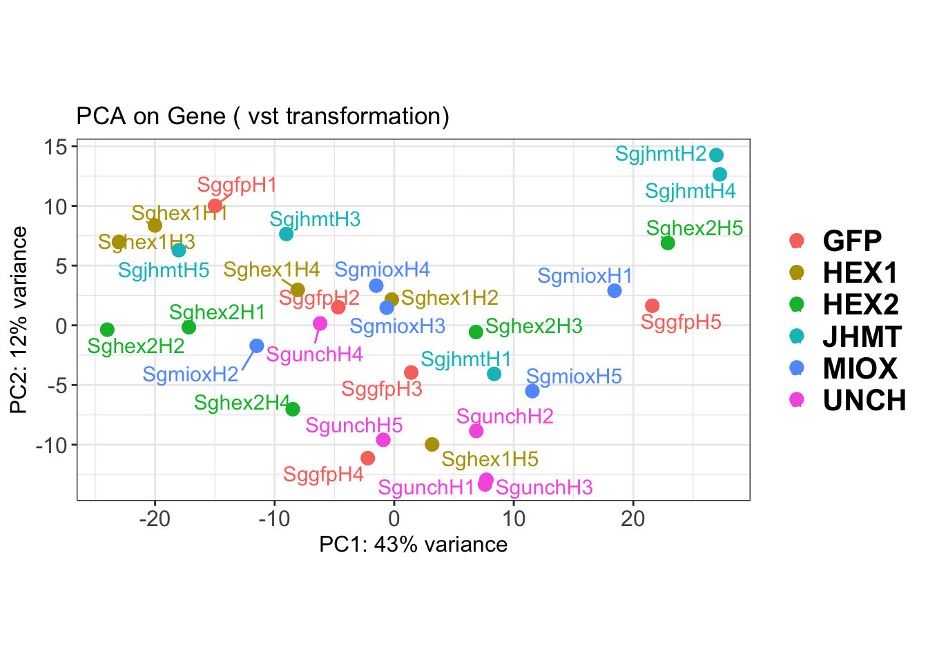
pca_results$PCA_Hull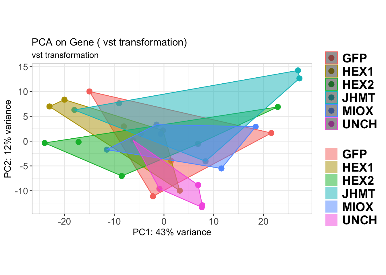
| Version | Author | Date |
|---|---|---|
| d7fa779 | Maeva TECHER | 2025-02-14 |
SVA
### SVA analysis to control for technical variation
dat <- counts(dds, normalized = TRUE)
idx <- rowMeans(dat) > 1
dat <- dat[idx, ]
mod <- model.matrix(~ Gene, colData(dds))
mod0 <- model.matrix(~ 1, colData(dds))
svseq <- svaseq(dat, mod, mod0)Number of significant surrogate variables is: 4
Iteration (out of 5 ):1 2 3 4 5 sva_plots <- create_sva_plots(svseq, dds, saveDir, intgroup = c("Tissue", "Gene"))
# Show stripcharts in the report
sva_plots$Stripcharts[[1]] # Show first stripchart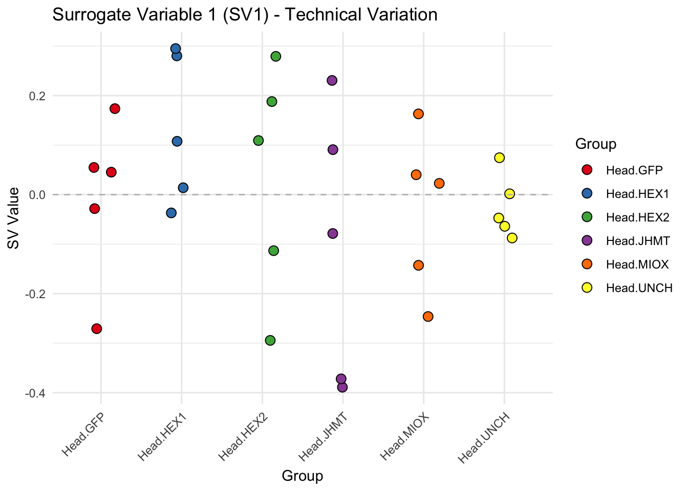
| Version | Author | Date |
|---|---|---|
| d7fa779 | Maeva TECHER | 2025-02-14 |
sva_plots$Stripcharts[[2]] # Show second stripchart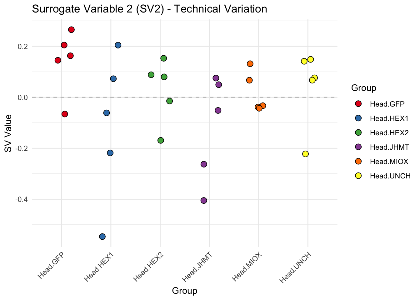
| Version | Author | Date |
|---|---|---|
| d7fa779 | Maeva TECHER | 2025-02-14 |
sva_plots$Stripcharts[[3]] # Show third stripchart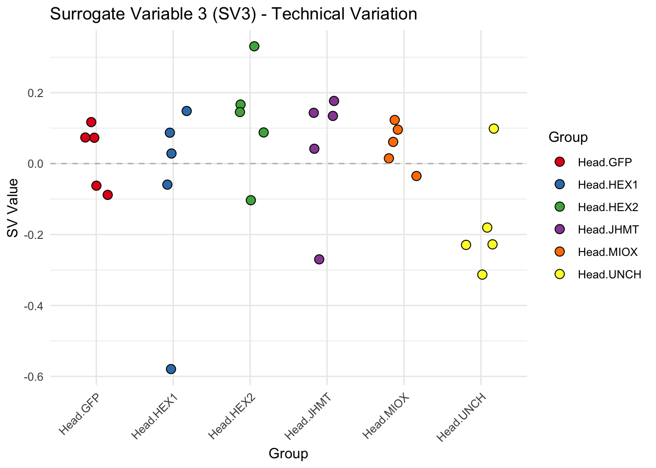
| Version | Author | Date |
|---|---|---|
| d7fa779 | Maeva TECHER | 2025-02-14 |
# Show scatter plots in the report
sva_plots$ScatterPlots[["1_2"]] # Show SV1 vs SV2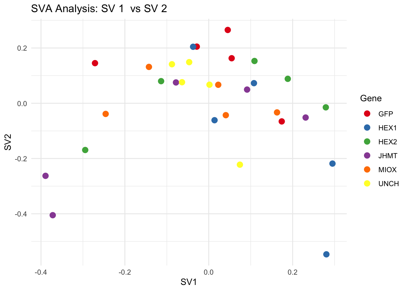
| Version | Author | Date |
|---|---|---|
| d7fa779 | Maeva TECHER | 2025-02-14 |
sva_plots$ScatterPlots[["1_3"]] # Show SV1 vs SV3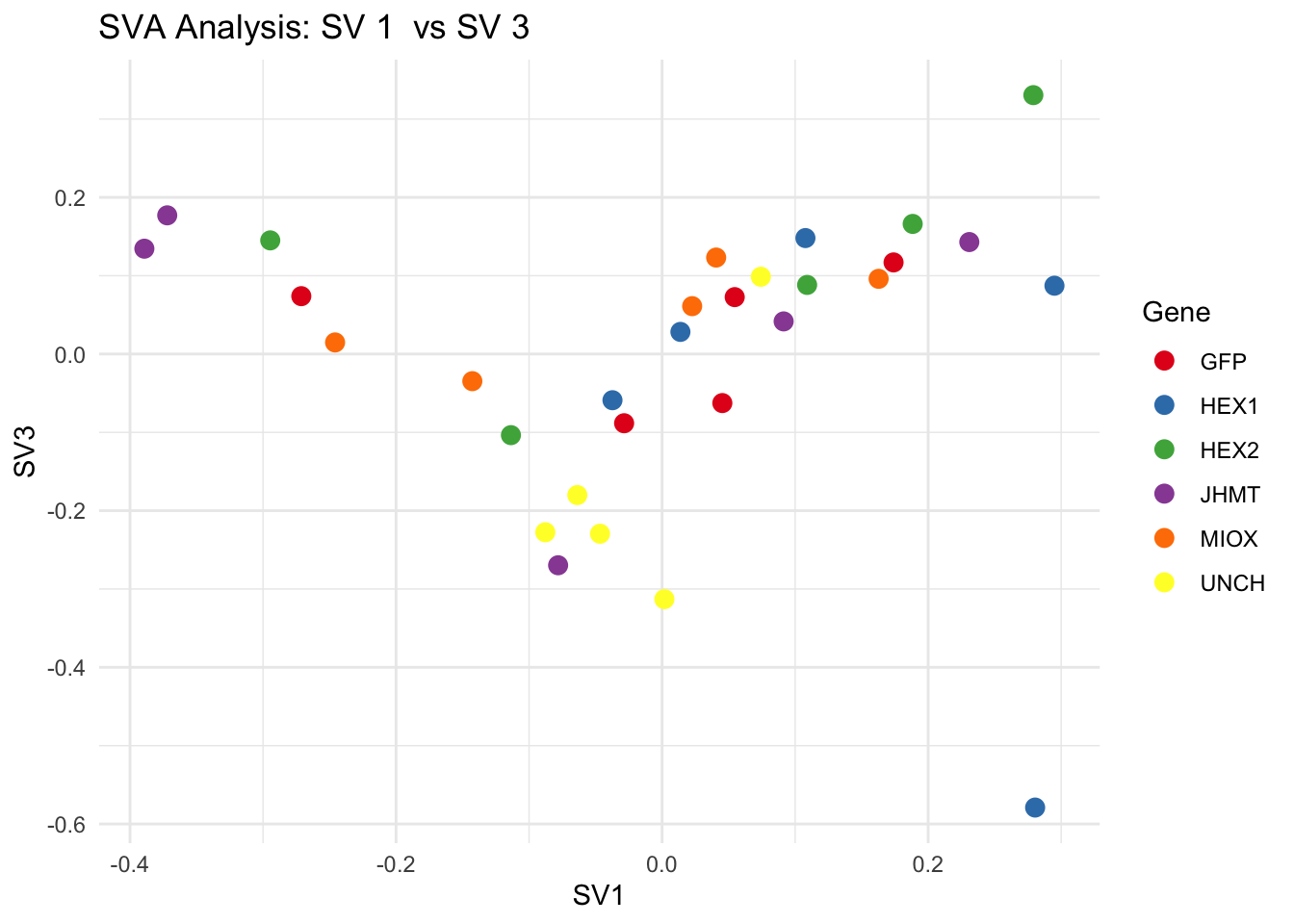
| Version | Author | Date |
|---|---|---|
| d7fa779 | Maeva TECHER | 2025-02-14 |
sva_plots$ScatterPlots[["2_3"]] # Show SV2 vs SV3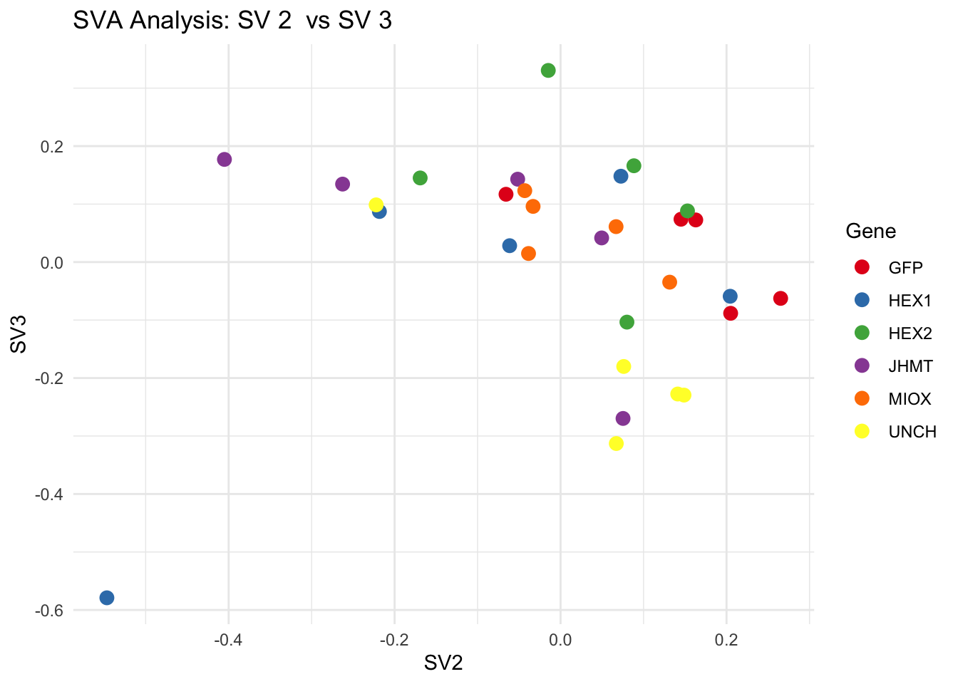
| Version | Author | Date |
|---|---|---|
| d7fa779 | Maeva TECHER | 2025-02-14 |
We rerun the DESeq2 model but this time including the
surrogate variable as a covariate, as we know that the modeled variation
is more likely explained by tissue and gene variation rather than batch
effects.
ddssva <- dds
ddssva$SV1 <- svseq$sv[,1]
ddssva$SV2 <- svseq$sv[,2]
ddssva$SV3 <- svseq$sv[,3]
design(ddssva) <- ~ SV1 + SV2 + SV3 + Gene
ddssva$Gene <- relevel(ddssva$Gene, ref = "GFP")
smallestGroupSize <- 5
keep <- rowSums(counts(ddssva) >= 10) >= smallestGroupSize
ddssva <- ddssva[keep,]
ddssva <- DESeq(ddssva)
ddssva <- ddssva[which(mcols(ddssva)$betaConv),] # remove non converging rows
### Extract results
message("Available contrasts are: ", paste(resultsNames(ddssva), collapse = ", "))
hex1 <- results(ddssva, name = "Gene_HEX1_vs_GFP", alpha = 0.05)
hex2 <- results(ddssva, name = "Gene_HEX2_vs_GFP", alpha = 0.05)
jhmt <- results(ddssva, name = "Gene_JHMT_vs_GFP", alpha = 0.05)
miox <- results(ddssva, name = "Gene_MIOX_vs_GFP", alpha = 0.05)
unch <- results(ddssva, name = "Gene_UNCH_vs_GFP", alpha = 0.05)Volcano plots and Heatmaps
First we create function to generate the plots we are interested to obtain and then run the whole pipeline for each gene.
# Define contrast_sets
hex1_samples <- c("SggfpH1","SggfpH2","SggfpH3","SggfpH4","SggfpH5",
"Sghex1H1","Sghex1H2","Sghex1H3","Sghex1H4","Sghex1H5")
hex2_samples <- c("SggfpH1","SggfpH2","SggfpH3","SggfpH4","SggfpH5",
"Sghex2H1","Sghex2H2","Sghex2H3","Sghex2H4","Sghex2H5")
jhmt_samples <- c("SggfpH1","SggfpH2","SggfpH3","SggfpH4","SggfpH5",
"SgjhmtH1","SgjhmtH2","SgjhmtH3","SgjhmtH4","SgjhmtH5")
miox_samples <- c("SggfpH1","SggfpH2","SggfpH3","SggfpH4","SggfpH5",
"SgmioxH1","SgmioxH2","SgmioxH3","SgmioxH4","SgmioxH5")
unch_samples <- c("SggfpH1","SggfpH2","SggfpH3","SggfpH4","SggfpH5",
"SgunchH1","SgunchH2","SgunchH3","SgunchH4","SgunchH5")
# Run full analysis
hex1_plots <- visualize_data(hex1, "HEX1_vs_GFP", hex1_samples)
hex2_plots <- visualize_data(hex2, "HEX2_vs_GFP", hex2_samples)
jhmt_plots <- visualize_data(jhmt, "JHMT_vs_GFP", jhmt_samples)
miox_plots <- visualize_data(miox, "MIOX_vs_GFP", miox_samples)
unch_plots <- visualize_data(unch, "UNCH_vs_GFP", unch_samples)
hex1_plots$volcano; hex1_plots$heatmap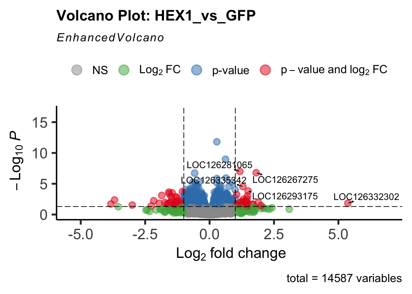
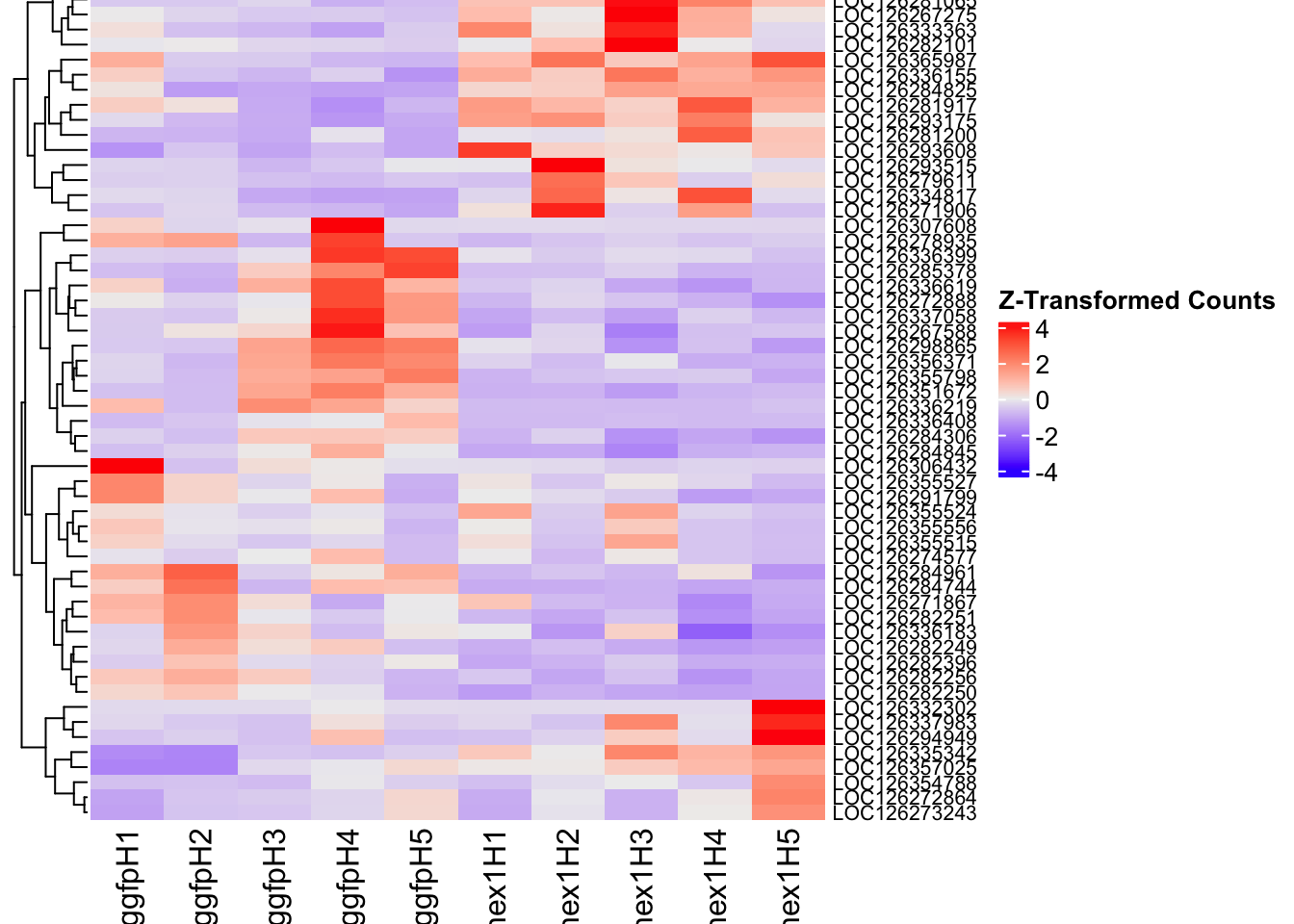
hex2_plots$volcano; hex2_plots$heatmap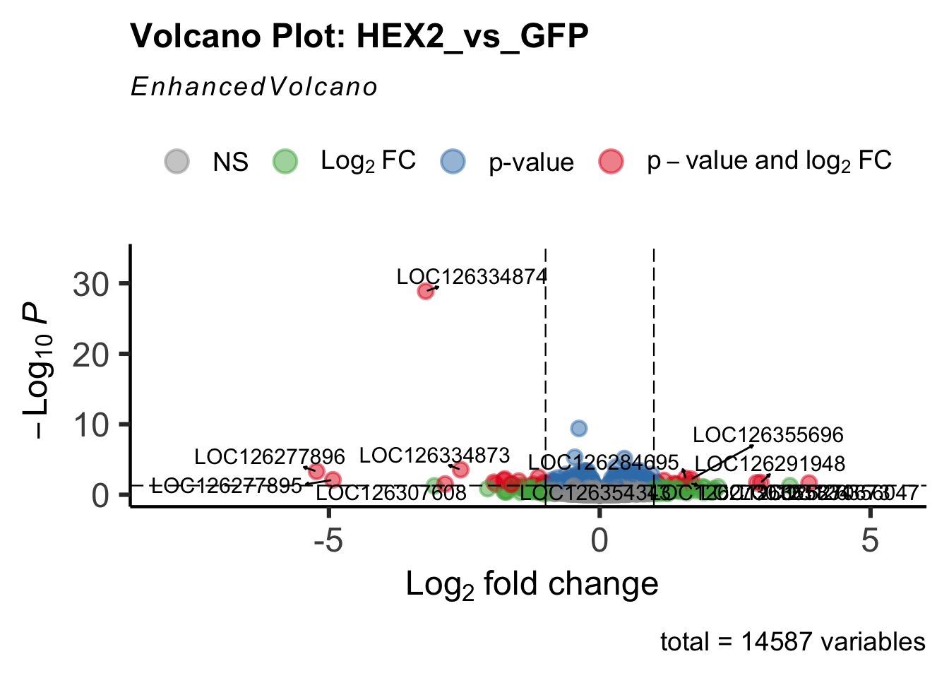
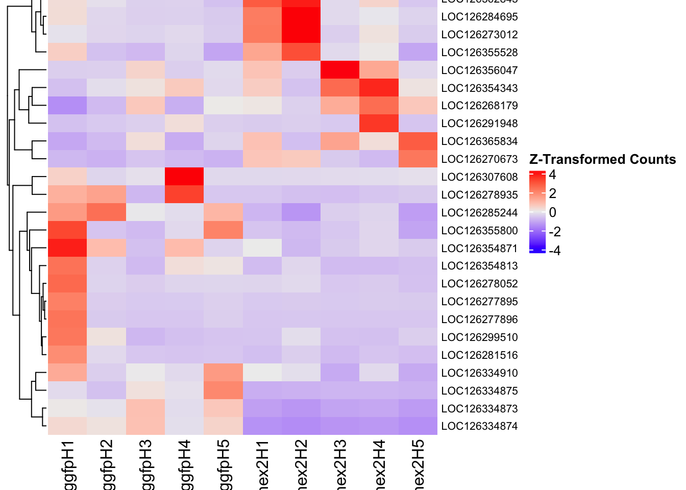
jhmt_plots$volcano; jhmt_plots$heatmap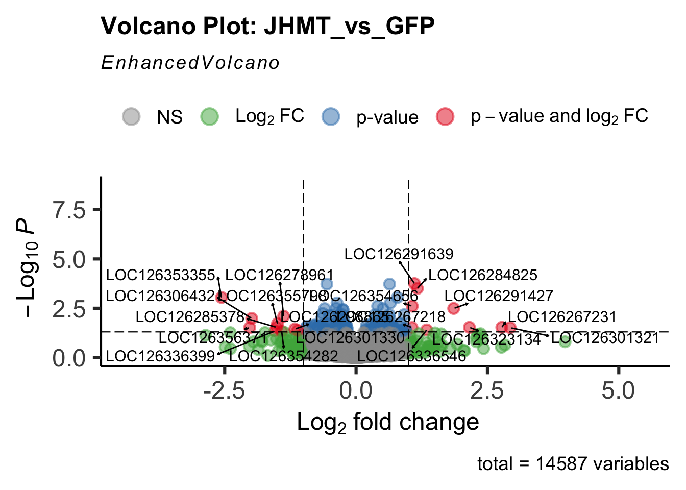
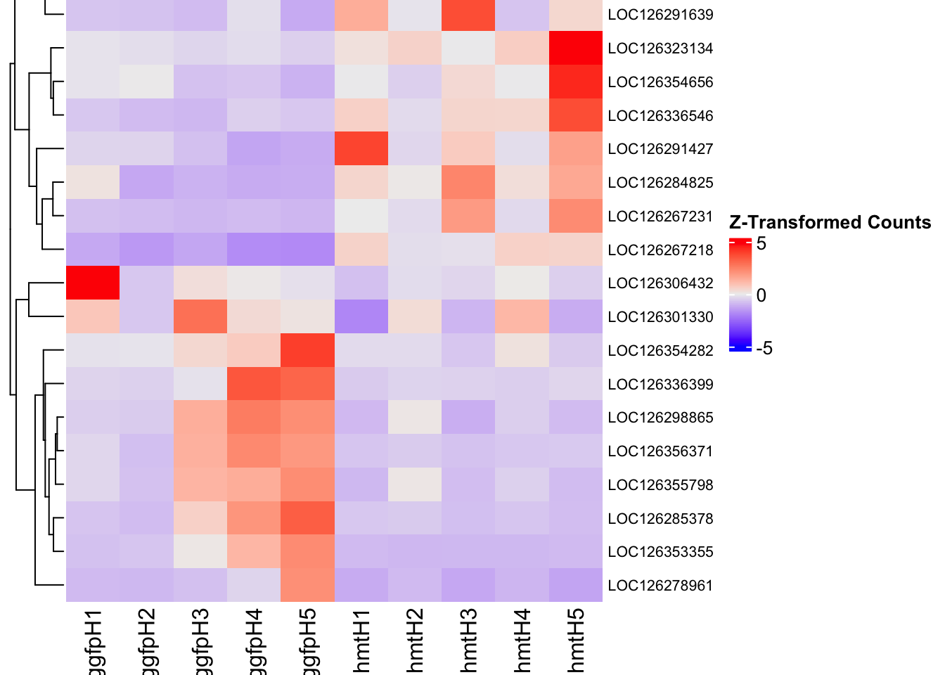
miox_plots$volcano; miox_plots$heatmap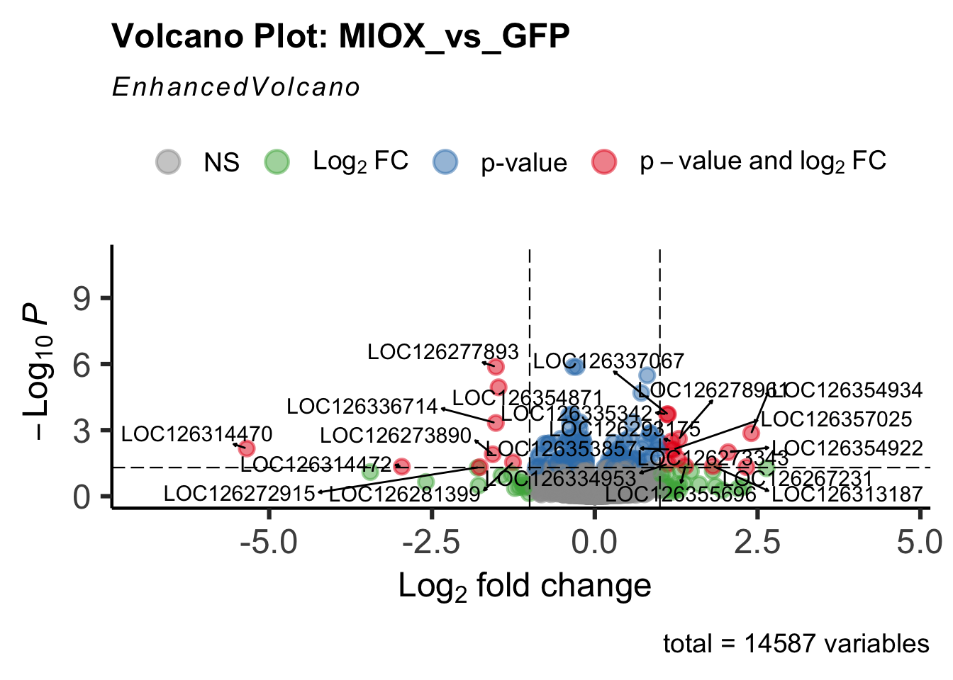
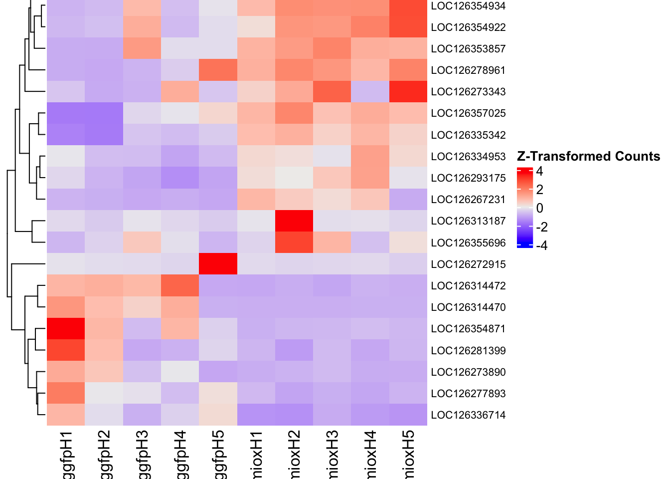
unch_plots$volcano; unch_plots$heatmap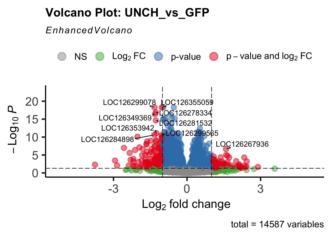
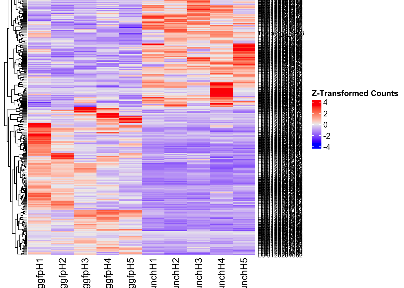
DEG tables
The following tables show the genes differentially expressed with at least an absolute log2fold change of > 1 considering head tissue only. Considering GFP as the reference state, upregulated genes in knockdown treatment in red and downregulated genes in knockdown treatment in blue. You can search for a gene of interest by writting a LOCID or description in the search bar or sort by column.
# Generate tables for each contrast
table_hex1 <- generate_deg_table(ddssva, "Gene_HEX1_vs_GFP", allspecies_df)
out of 14587 with nonzero total read count
adjusted p-value < 0.05
LFC > 0 (up) : 432, 3%
LFC < 0 (down) : 463, 3.2%
outliers [1] : 0, 0%
low counts [2] : 2546, 17%
(mean count < 31)
[1] see 'cooksCutoff' argument of ?results
[2] see 'independentFiltering' argument of ?resultsTotal DEGs p-value < 0.05 and absolute logFoldChange > 1: 58LFC > 1 (up) : 26 (44.83%)LFC < -1 (down) : 32 (55.17%)table_hex1$kable_tabletable_hex2 <- generate_deg_table(ddssva, "Gene_HEX2_vs_GFP", allspecies_df)
out of 14587 with nonzero total read count
adjusted p-value < 0.05
LFC > 0 (up) : 171, 1.2%
LFC < 0 (down) : 287, 2%
outliers [1] : 0, 0%
low counts [2] : 2263, 16%
(mean count < 26)
[1] see 'cooksCutoff' argument of ?results
[2] see 'independentFiltering' argument of ?resultsTotal DEGs p-value < 0.05 and absolute logFoldChange > 1: 26LFC > 1 (up) : 11 (42.31%)LFC < -1 (down) : 15 (57.69%)table_hex2$kable_tabletable_jhmt <- generate_deg_table(ddssva, "Gene_JHMT_vs_GFP", allspecies_df)
out of 14587 with nonzero total read count
adjusted p-value < 0.05
LFC > 0 (up) : 73, 0.5%
LFC < 0 (down) : 106, 0.73%
outliers [1] : 0, 0%
low counts [2] : 1980, 14%
(mean count < 22)
[1] see 'cooksCutoff' argument of ?results
[2] see 'independentFiltering' argument of ?resultsTotal DEGs p-value < 0.05 and absolute logFoldChange > 1: 19LFC > 1 (up) : 9 (47.37%)LFC < -1 (down) : 10 (52.63%)table_jhmt$kable_tabletable_miox <- generate_deg_table(ddssva, "Gene_MIOX_vs_GFP", allspecies_df)
out of 14587 with nonzero total read count
adjusted p-value < 0.05
LFC > 0 (up) : 61, 0.42%
LFC < 0 (down) : 112, 0.77%
outliers [1] : 0, 0%
low counts [2] : 3677, 25%
(mean count < 60)
[1] see 'cooksCutoff' argument of ?results
[2] see 'independentFiltering' argument of ?resultsTotal DEGs p-value < 0.05 and absolute logFoldChange > 1: 21LFC > 1 (up) : 13 (61.9%)LFC < -1 (down) : 8 (38.1%)table_miox$kable_tabletable_unch <- generate_deg_table(ddssva, "Gene_UNCH_vs_GFP", allspecies_df)
out of 14587 with nonzero total read count
adjusted p-value < 0.05
LFC > 0 (up) : 1355, 9.3%
LFC < 0 (down) : 1860, 13%
outliers [1] : 0, 0%
low counts [2] : 283, 1.9%
(mean count < 8)
[1] see 'cooksCutoff' argument of ?results
[2] see 'independentFiltering' argument of ?resultsTotal DEGs p-value < 0.05 and absolute logFoldChange > 1: 266LFC > 1 (up) : 121 (45.49%)LFC < -1 (down) : 145 (54.51%)table_unch$kable_tableSummary and Overlap
# Summarize DEGs for all contrasts
deg_summary <- bind_rows(
summarize_deg_counts(table_hex1, "HEX1 vs GFP"),
summarize_deg_counts(table_hex2, "HEX2 vs GFP"),
summarize_deg_counts(table_jhmt, "JHMT vs GFP"),
summarize_deg_counts(table_miox, "MIOX vs GFP"),
summarize_deg_counts(table_unch, "UNCH vs GFP")
)
# Display table using kable with styling
deg_summary %>%
kable("html", escape = FALSE, col.names = gsub("_", " ", names(.))) %>%
kable_styling("striped", full_width = TRUE) %>%
column_spec(2, color = "red", bold = TRUE) %>% # Upregulated in red
column_spec(3, color = "blue", bold = TRUE) %>% # Downregulated in blue
add_header_above(c("Summary of DEGs" = 3)) %>%
row_spec(0, bold = TRUE)| Contrast | Upregulated | Downregulated |
|---|---|---|
| HEX1 vs GFP | 23 | 30 |
| HEX2 vs GFP | 11 | 15 |
| JHMT vs GFP | 9 | 9 |
| MIOX vs GFP | 12 | 6 |
| UNCH vs GFP | 117 | 142 |
# Define the list of RNAi contrasts
contrast_list <- c("HEX1_vs_GFP", "HEX2_vs_GFP", "JHMT_vs_GFP",
"MIOX_vs_GFP", "UNCH_vs_GFP")
# Initialize empty lists for storing Head-specific DEGs for each contrast
venn_data_up <- list()
venn_data_down <- list()
venn_data_all <- list()
# Function to load Head-specific DEGs for a given set of contrasts
load_deg_contrasts_head <- function(contrast_list) {
degs_up <- list()
degs_down <- list()
degs_all <- list()
for (contrast in contrast_list) {
deg_file <- file.path(workDir, "DEG_results/RNAi/Head_no_rRNA/", contrast, paste0("DEG_sigresults_", contrast, ".csv"))
if (!file.exists(deg_file)) {
message(paste("File missing for contrast:", contrast))
next # Skip if the file doesn't exist
}
deg_data <- read.csv(deg_file, stringsAsFactors = FALSE)
# Convert row names to a column if necessary
if ("X" %in% colnames(deg_data)) {
colnames(deg_data)[colnames(deg_data) == "X"] <- "GeneID"
}
# Check if data is empty
if (nrow(deg_data) == 0) {
message(paste("No data for contrast:", contrast))
next
}
# Select significant DEGs (Up, Down, All)
degs_up[[contrast]] <- deg_data %>%
filter(padj < 0.05 & log2FoldChange >= 1) %>%
pull(GeneID) # Extract GeneID column
degs_down[[contrast]] <- deg_data %>%
filter(padj < 0.05 & log2FoldChange <= -1) %>%
pull(GeneID) # Extract GeneID column
degs_all[[contrast]] <- deg_data %>%
filter(padj < 0.05 & abs(log2FoldChange) >= 1) %>%
pull(GeneID) # Extract GeneID column
}
return(list(up = degs_up, down = degs_down, all = degs_all))
}
# Load DEG data for the defined contrasts (Head tissue only)
venn_data_contrasts <- load_deg_contrasts_head(contrast_list)
# Prepare the data for the Venn diagrams
venn_data_up <- venn_data_contrasts$up
venn_data_down <- venn_data_contrasts$down
venn_data_all <- venn_data_contrasts$all
# Function to display Venn diagram and corresponding datatable
display_venn_with_datatable <- function(venn_data, title, allspecies_df) {
# Calculate the overlapping genes
overlap_genes <- Reduce(intersect, venn_data)
# Create a data frame for the overlapping genes
overlap_df <- data.frame(GeneID = overlap_genes)
# Merge to get species information
meta_brock_df <- merge(overlap_df, allspecies_df, by = "GeneID", all.x = TRUE)
# Generate the Venn diagram
venn_plot <- venn.diagram(
x = venn_data,
category.names = contrast_list,
filename = NULL,
output = TRUE,
fill = c("orange", "red", "blue", "purple", "green"), # Adjust colors for contrasts
alpha = 0.5,
cex = 2,
cat.cex = 0,
main = title,
main.cex = 1.2
)
# Clear the plotting area before drawing
grid.newpage()
grid.draw(venn_plot)
# Create a custom legend
legend_labels <- contrast_list
legend_colors <- c("orange", "red", "blue", "purple", "green")
# Positioning the legend
legend_x <- unit(0.85, "npc") # Adjust x position
legend_y <- unit(0.2, "npc") # Adjust y position
# Draw the legend
for (i in 1:length(legend_labels)) {
grid.rect(x = legend_x, y = legend_y - unit((i - 1) * 0.05, "npc"),
width = unit(0.02, "npc"), height = unit(0.02, "npc"),
gp = gpar(fill = legend_colors[i], col = NA))
grid.text(label = legend_labels[i], x = legend_x + unit(0.05, "npc"),
y = legend_y - unit((i - 1) * 0.05, "npc"),
just = "left", gp = gpar(cex = 0.8))
}
# Display the merged overlapping genes table with datatable
datatable(meta_brock_df, options = list(
pageLength = 10,
scrollX = TRUE,
autoWidth = TRUE,
searchHighlight = TRUE
),
rownames = FALSE,
escape = FALSE
) %>%
formatStyle(
'Species', target = 'cell',
fontStyle = 'italic'
) %>%
formatStyle(
columns = names(meta_brock_df),
target = 'row',
color = styleEqual(c("red", "blue", "black"), c("red", "blue", "black")),
fontWeight = styleEqual(c("bold", "normal"), c("bold", "normal")),
backgroundColor = styleEqual(c("red", "blue", "black"), c("white", "white", "white"))
)
}
# Display the Venn diagram and datatable for **Head Upregulated DEGs** across contrasts
display_venn_with_datatable(venn_data_up, "Venn Diagram of Head Upregulated DEGs - RNAi Contrasts", allspecies_df)
| Version | Author | Date |
|---|---|---|
| b540a1e | Maeva TECHER | 2025-02-27 |
# Display the Venn diagram and datatable for **Head Downregulated DEGs** across contrasts
display_venn_with_datatable(venn_data_down, "Venn Diagram of Head Downregulated DEGs - RNAi Contrasts", allspecies_df)
| Version | Author | Date |
|---|---|---|
| b540a1e | Maeva TECHER | 2025-02-27 |
# Display the Venn diagram and datatable for **All Significant DEGs in Head Tissue**
display_venn_with_datatable(venn_data_all, "Venn Diagram of All Significant DEGs in Head Tissue - RNAi Contrasts", allspecies_df)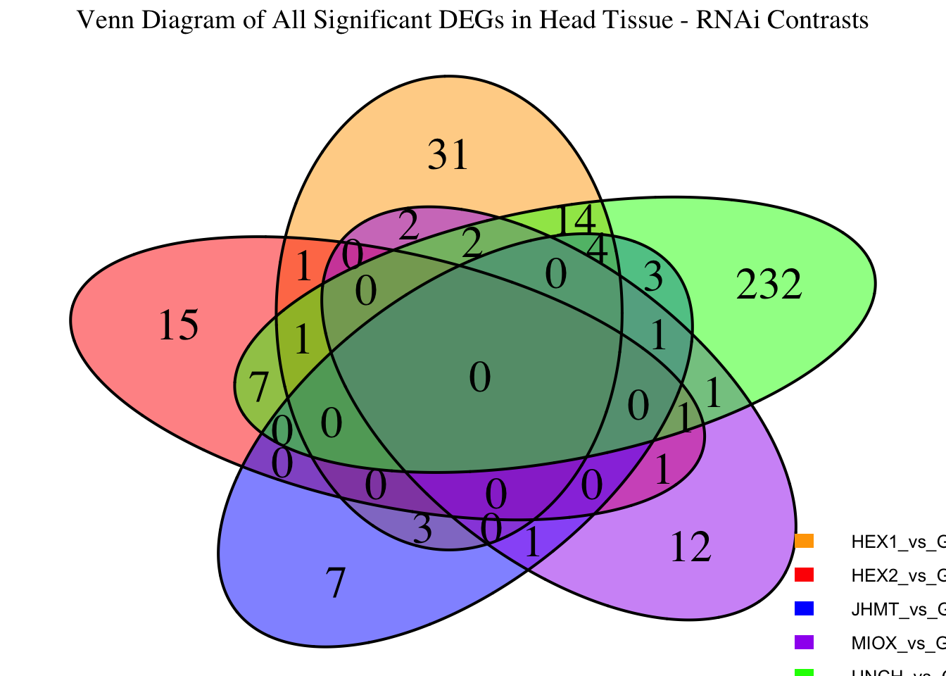
| Version | Author | Date |
|---|---|---|
| b540a1e | Maeva TECHER | 2025-02-27 |
GO and KEGG enrichment
#enrich_data(hex1, "Hex1_vs_GFP", hex1_samples)
#enrich_data(hex2, "Hex2_vs_GFP", hex2_samples)
#enrich_data(jhmt, "JHMT_vs_GFP", jhmt_samples)
#enrich_data(miox, "MIOX_vs_GFP", miox_samples)
#enrich_data(unch, "UNCH_vs_GFP", unch_samples)Thorax tissue
Minor changes here are made compared to the DESeq2 results regarding the importation of samples to transform into a matrix. Sample names are structured as follow: {Sg}{gene}{#} {Sg} = Schistocerca gregaria {gene} = gene abbreviation gfp, hex1, hex2, jhmt, miox and unch T{#} = biological replicate
saveDir <- paste0(workDir,"/DEG_results/RNAi/Thorax_no_rRNA")
dir.create(saveDir)
### Prepare Sample CSV file #####
samples <- read.delim(file.path(workDir, "list/RNAi/Thorax_RNAisample_list.csv"), sep = ",", row.names = 1, header = TRUE)
files <- file.path(workDir, "readcounts/RNAi/", samples$Tissue, samples$Filename)
names(files) <- row.names(samples)
if (all(file.exists(files))) {
message("All the files exist!")
} else {
warning("Some files are missing!")
}All the files exist!### Create count sample matrix
cts <- map_dfc(files, function(sample) {
data_count <- read.delim(sample, sep = "\t", header = FALSE)
col_name <- gsub("_counts.txt", "", basename(sample))
setNames(data.frame(data_count[, 2]), col_name)
})
row_get <- read.delim(files[1], sep = "\t", row.names = 1, header = F) # Get proper row names
rownames(cts) <- rownames(row_get)
rm(row_get) # remove unused object from memoryWhile for bulk RNAseq on head and thorax for all species, the DEGs model was made between isolated and crowded individuals (with isolated as the reference state), here, the DEG analysis will be carried between GFP knock-down nymphs (as reference state) vs Hexamerins / Juvenile Hormones / Uncharacterized proteins.
### Build DESeq2 Object
dds <- DESeqDataSetFromMatrix(countData = cts,
colData = samples,
design = ~ Gene)
dds$Gene <- relevel(dds$Gene, ref = "GFP")
smallestGroupSize <- 5
keep <- rowSums(counts(dds) >= 10) >= smallestGroupSize
dds <- dds[keep,]
loci_to_exclude <- readLines(file.path(workDir, "list/excluded_loci/gregaria_rrna_list.txt"))
dds <- dds[!(rownames(dds) %in% loci_to_exclude), ]
dds <- DESeq(dds)Normalization and PCA
# Plot PCA and investigate quality metrics
vsd <- vst(dds, blind=T)
pca_results <- create_pca_plots(norm.dds = vsd, saveDir, transformation = "vst", intgroup = "Gene")
pca_results$PCA_Labelled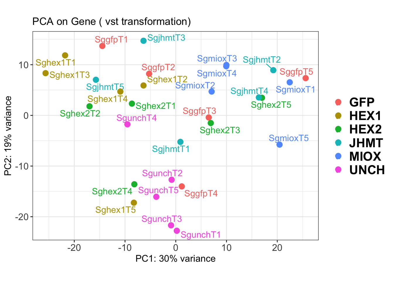
| Version | Author | Date |
|---|---|---|
| d7fa779 | Maeva TECHER | 2025-02-14 |
pca_results$PCA_Hull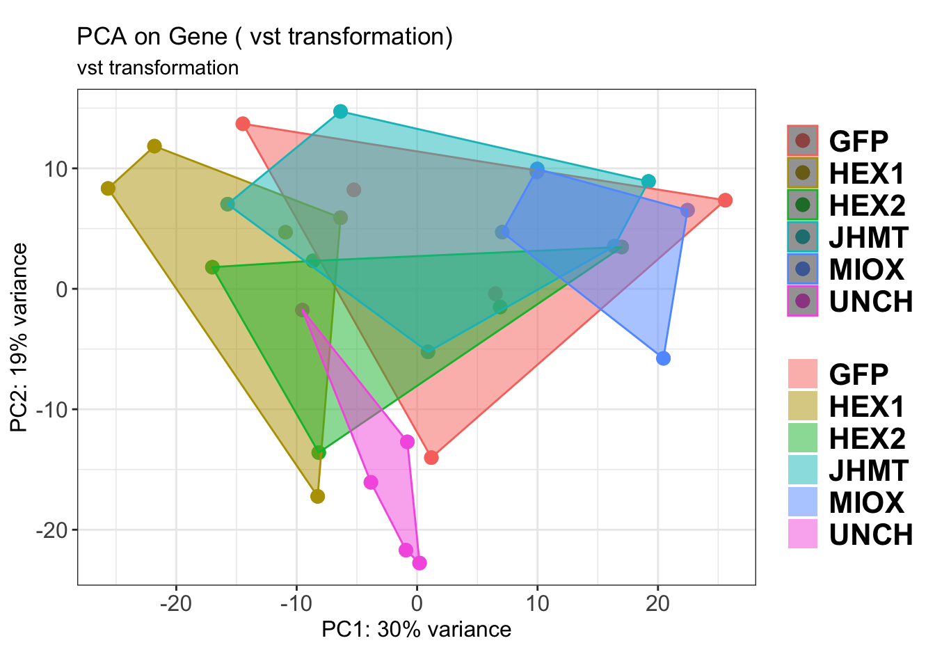
| Version | Author | Date |
|---|---|---|
| d7fa779 | Maeva TECHER | 2025-02-14 |
SVA
### SVA analysis to control for technical variation
dat <- counts(dds, normalized = TRUE)
idx <- rowMeans(dat) > 1
dat <- dat[idx, ]
mod <- model.matrix(~ Gene, colData(dds))
mod0 <- model.matrix(~ 1, colData(dds))
svseq <- svaseq(dat, mod, mod0)Number of significant surrogate variables is: 5
Iteration (out of 5 ):1 2 3 4 5 sva_plots <- create_sva_plots(svseq, dds, saveDir, intgroup = c("Tissue", "Gene"))
# Show stripcharts in the report
sva_plots$Stripcharts[[1]] # Show first stripchart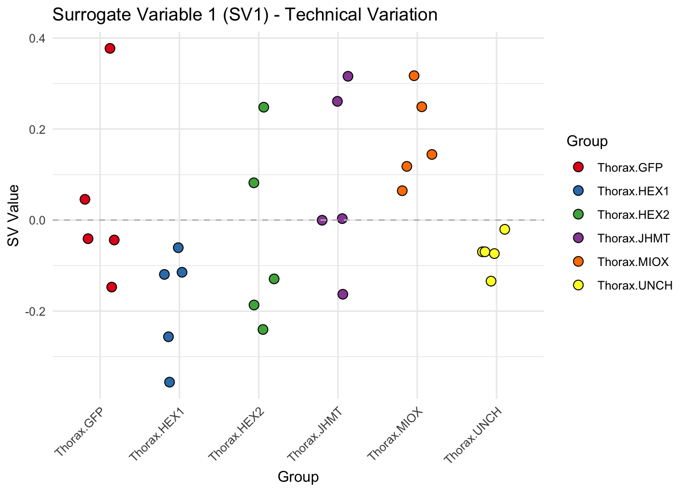
| Version | Author | Date |
|---|---|---|
| d7fa779 | Maeva TECHER | 2025-02-14 |
sva_plots$Stripcharts[[2]] # Show second stripchart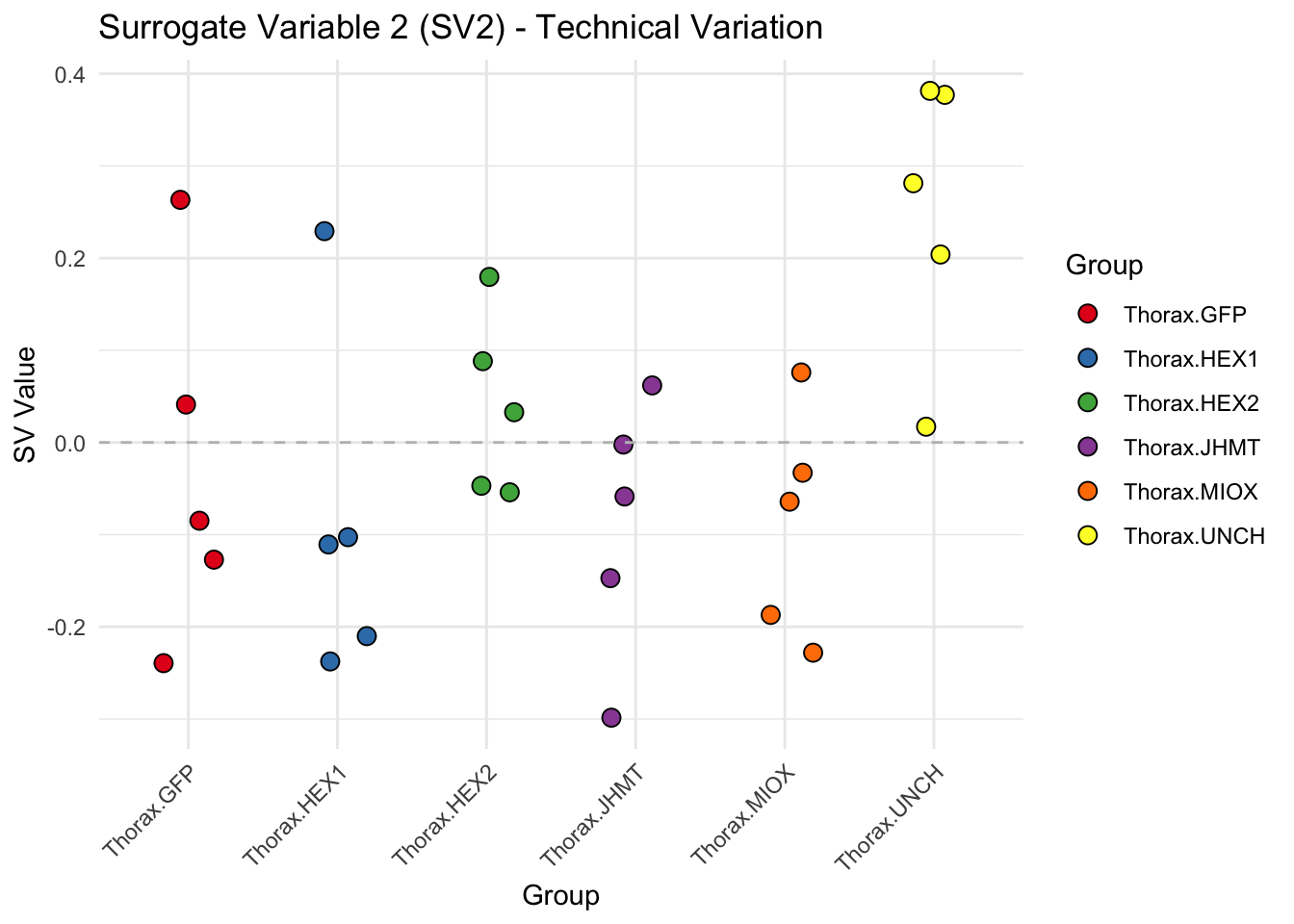
| Version | Author | Date |
|---|---|---|
| d7fa779 | Maeva TECHER | 2025-02-14 |
sva_plots$Stripcharts[[3]] # Show third stripchart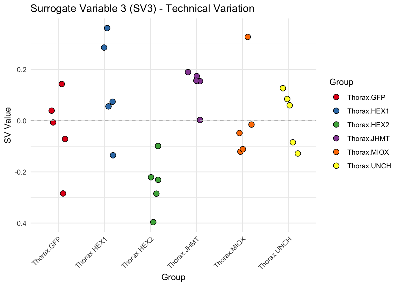
| Version | Author | Date |
|---|---|---|
| d7fa779 | Maeva TECHER | 2025-02-14 |
# Show scatter plots in the report
sva_plots$ScatterPlots[["1_2"]] # Show SV1 vs SV2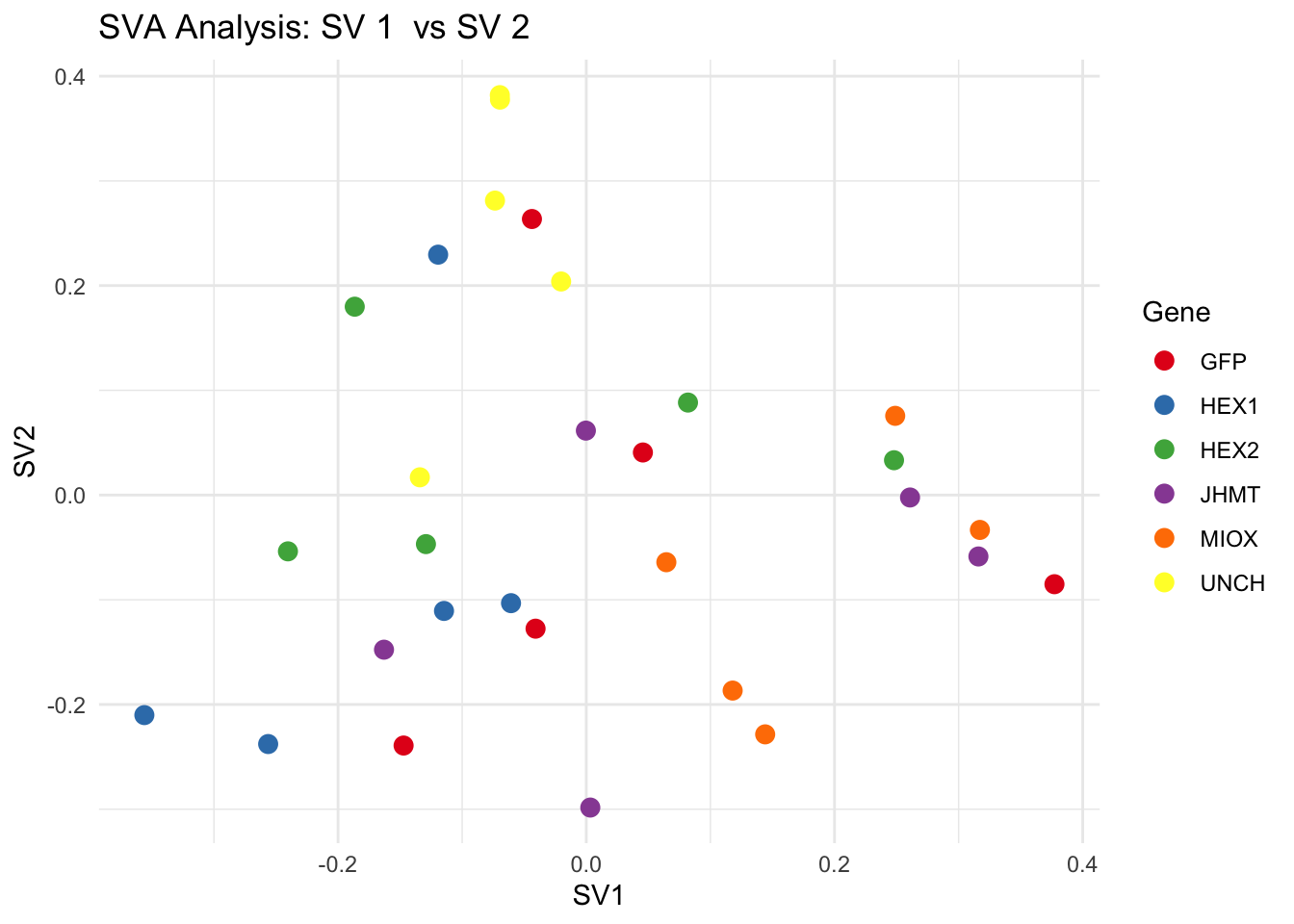
| Version | Author | Date |
|---|---|---|
| d7fa779 | Maeva TECHER | 2025-02-14 |
sva_plots$ScatterPlots[["1_3"]] # Show SV1 vs SV3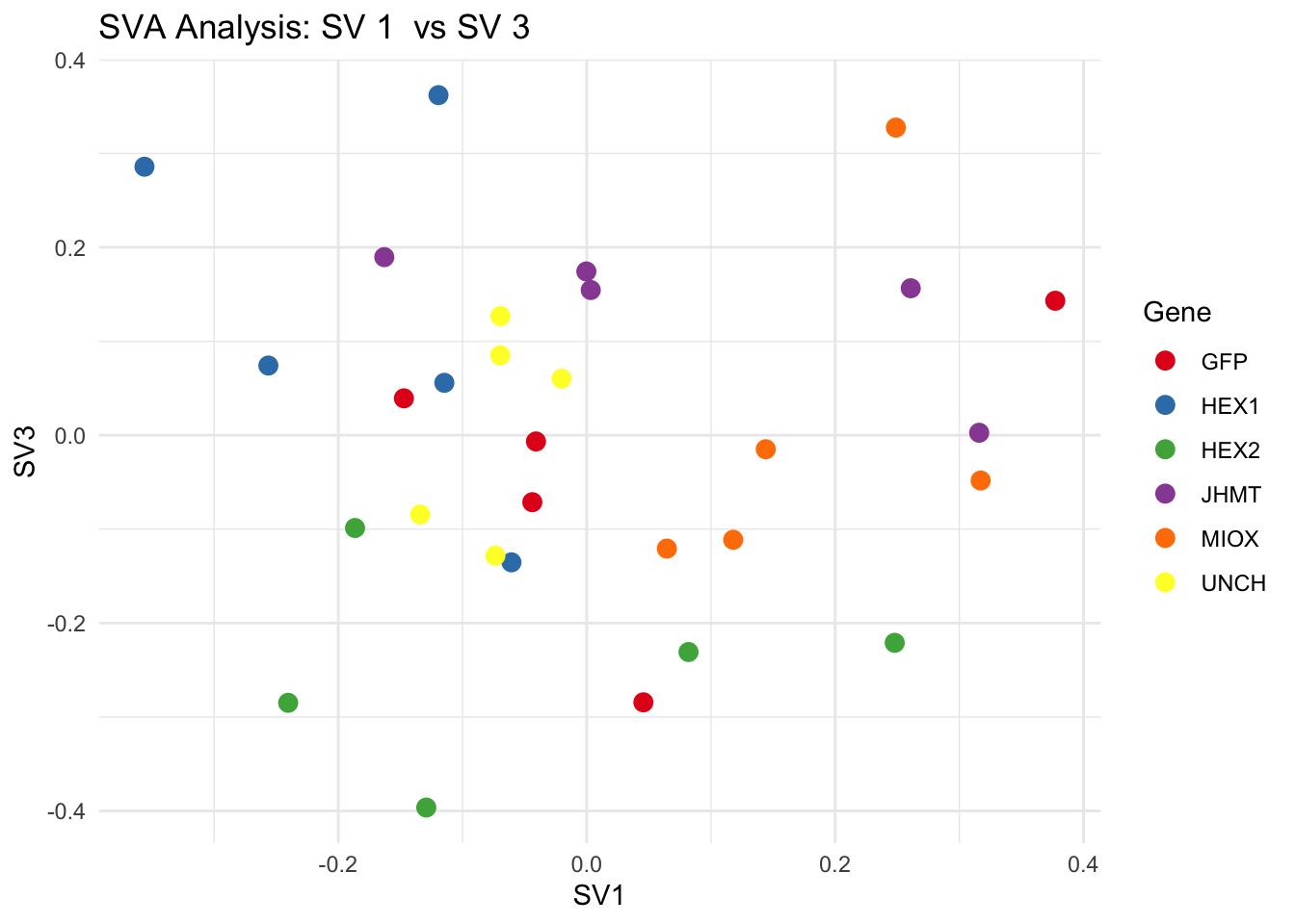
| Version | Author | Date |
|---|---|---|
| d7fa779 | Maeva TECHER | 2025-02-14 |
sva_plots$ScatterPlots[["2_3"]] # Show SV2 vs SV3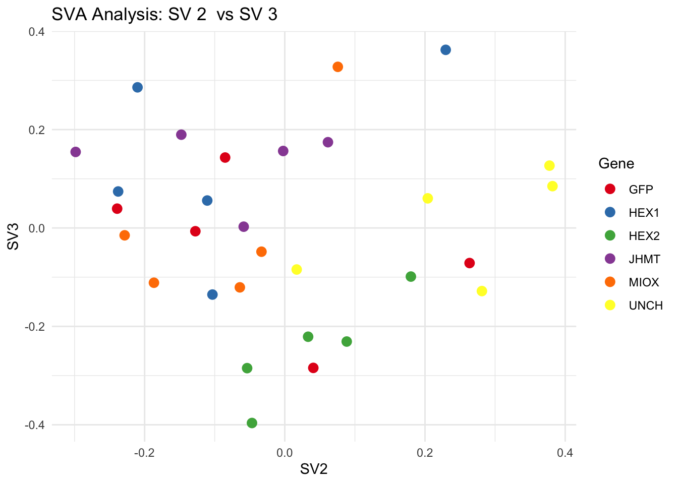
| Version | Author | Date |
|---|---|---|
| d7fa779 | Maeva TECHER | 2025-02-14 |
We rerun the DESeq2 model but this time including the
surrogate variable as a covariate, as we know that the modeled variation
is more likely explained by tissue and gene variation rather than batch
effects.
ddssva <- dds
ddssva$SV1 <- svseq$sv[,1]
ddssva$SV2 <- svseq$sv[,2]
ddssva$SV3 <- svseq$sv[,3]
design(ddssva) <- ~ SV1 + SV2 + SV3 + Gene
ddssva$Gene <- relevel(ddssva$Gene, ref = "GFP")
smallestGroupSize <- 5
keep <- rowSums(counts(ddssva) >= 10) >= smallestGroupSize
ddssva <- ddssva[keep,]
ddssva <- DESeq(ddssva)
ddssva <- ddssva[which(mcols(ddssva)$betaConv),] # remove non converging rows
### Extract results
message("Available contrasts are: ", paste(resultsNames(ddssva), collapse = ", "))
hex1 <- results(ddssva, name = "Gene_HEX1_vs_GFP", alpha = 0.05)
hex2 <- results(ddssva, name = "Gene_HEX2_vs_GFP", alpha = 0.05)
jhmt <- results(ddssva, name = "Gene_JHMT_vs_GFP", alpha = 0.05)
miox <- results(ddssva, name = "Gene_MIOX_vs_GFP", alpha = 0.05)
unch <- results(ddssva, name = "Gene_UNCH_vs_GFP", alpha = 0.05)Volcano plots and Heatmaps
First we create function to generate the plots we are interested to obtain and then run the whole pipeline for each gene.
# Define contrast_sets
hex1_samples <- c("SggfpT1","SggfpT2","SggfpT3","SggfpT4","SggfpT5",
"Sghex1T1","Sghex1T2","Sghex1T3","Sghex1T4","Sghex1T5")
hex2_samples <- c("SggfpT1","SggfpT2","SggfpT3","SggfpT4","SggfpT5",
"Sghex2T1","Sghex2T2","Sghex2T3","Sghex2T4","Sghex2T5")
jhmt_samples <- c("SggfpT1","SggfpT2","SggfpT3","SggfpT4","SggfpT5",
"SgjhmtT1","SgjhmtT2","SgjhmtT3","SgjhmtT4","SgjhmtT5")
miox_samples <- c("SggfpT1","SggfpT2","SggfpT3","SggfpT4","SggfpT5",
"SgmioxT1","SgmioxT2","SgmioxT3","SgmioxT4","SgmioxT5")
unch_samples <- c("SggfpT1","SggfpT2","SggfpT3","SggfpT4","SggfpT5",
"SgunchT1","SgunchT2","SgunchT3","SgunchT4","SgunchT5")
# Run full analysis
hex1_plots <- visualize_data(hex1, "HEX1_vs_GFP", hex1_samples)
hex2_plots <- visualize_data(hex2, "HEX2_vs_GFP", hex2_samples)
jhmt_plots <- visualize_data(jhmt, "JHMT_vs_GFP", jhmt_samples)
miox_plots <- visualize_data(miox, "MIOX_vs_GFP", miox_samples)
unch_plots <- visualize_data(unch, "UNCH_vs_GFP", unch_samples)
hex1_plots$volcano; hex1_plots$heatmap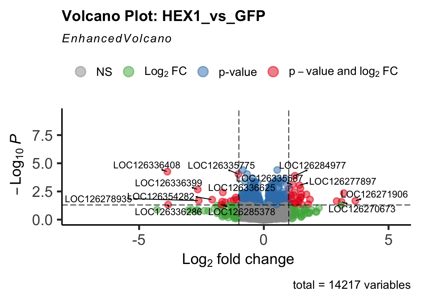
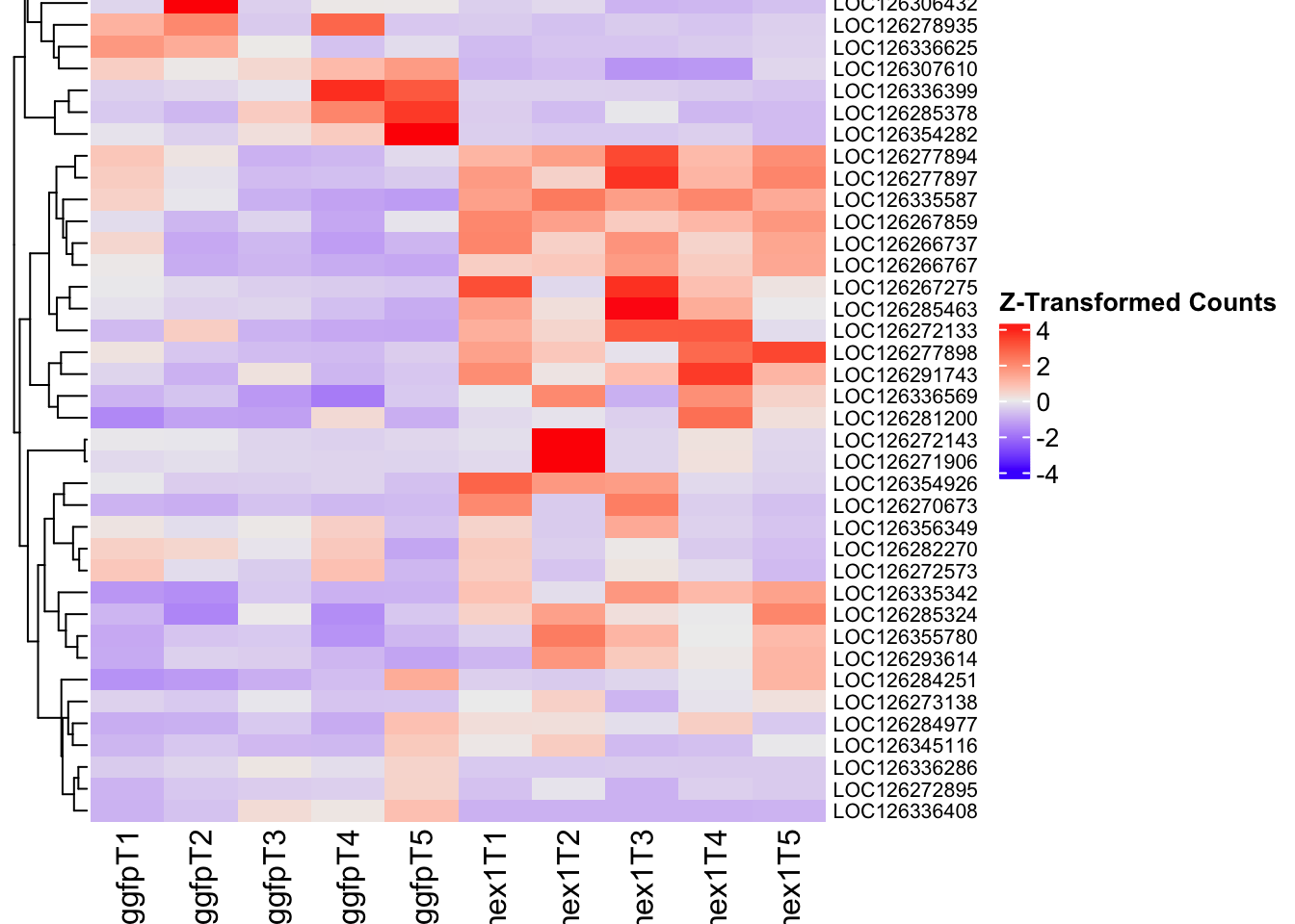
hex2_plots$volcano; hex2_plots$heatmap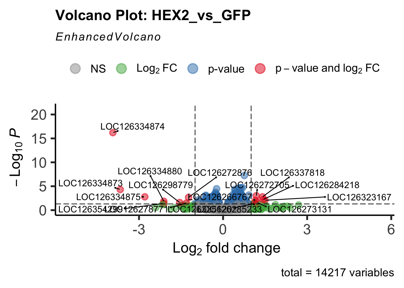
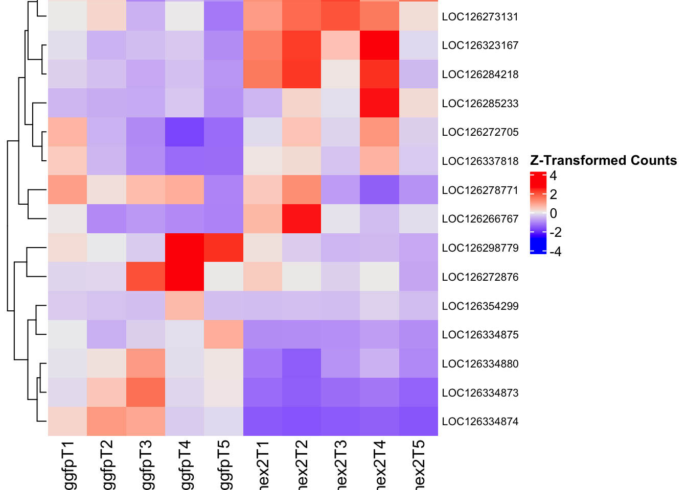
jhmt_plots$volcano; jhmt_plots$heatmap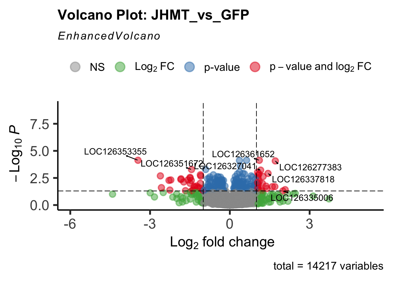
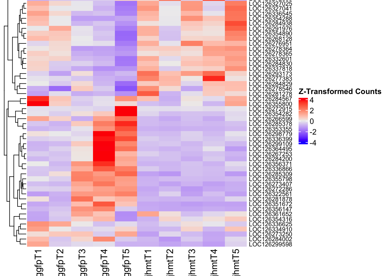
miox_plots$volcano; miox_plots$heatmap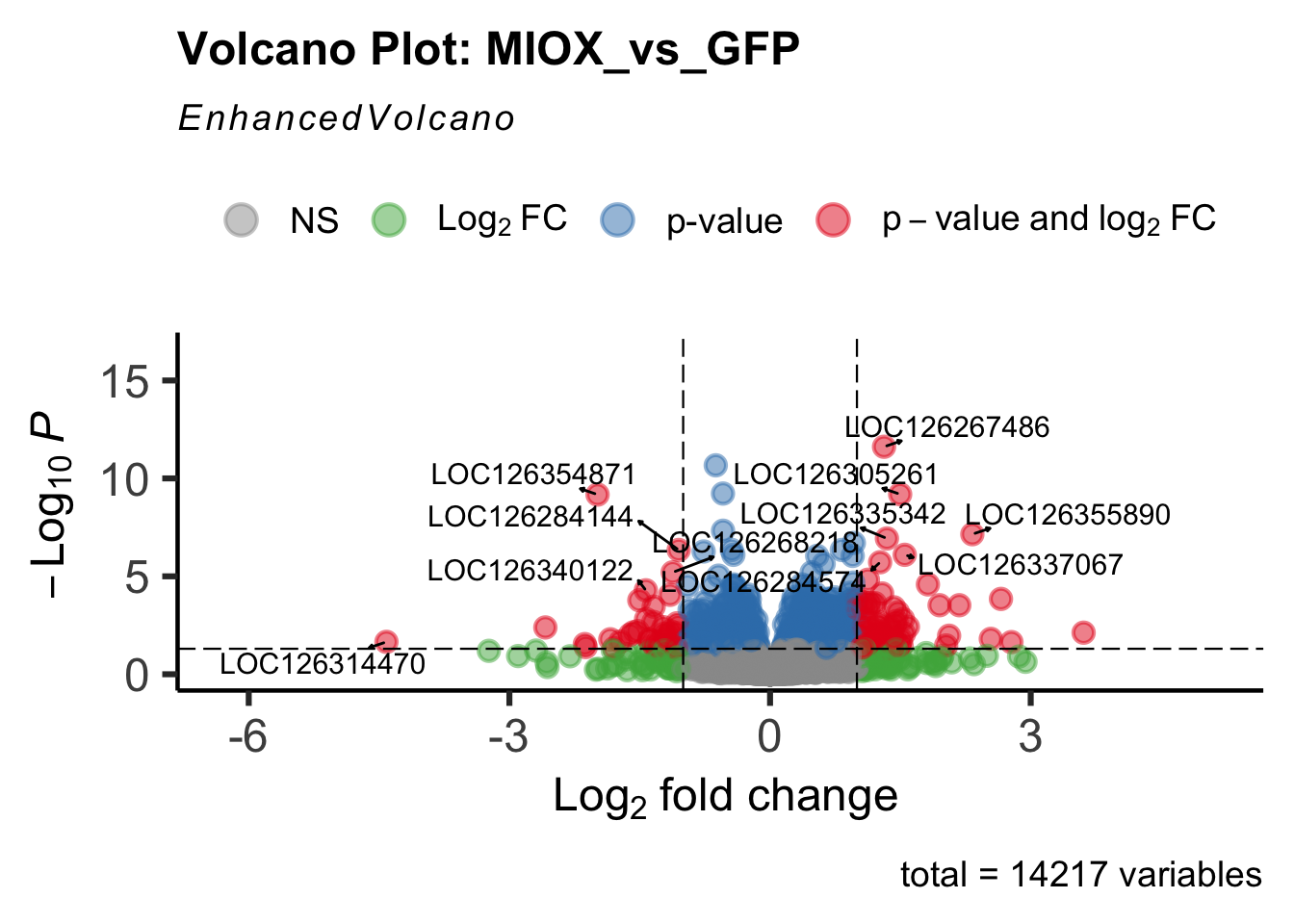
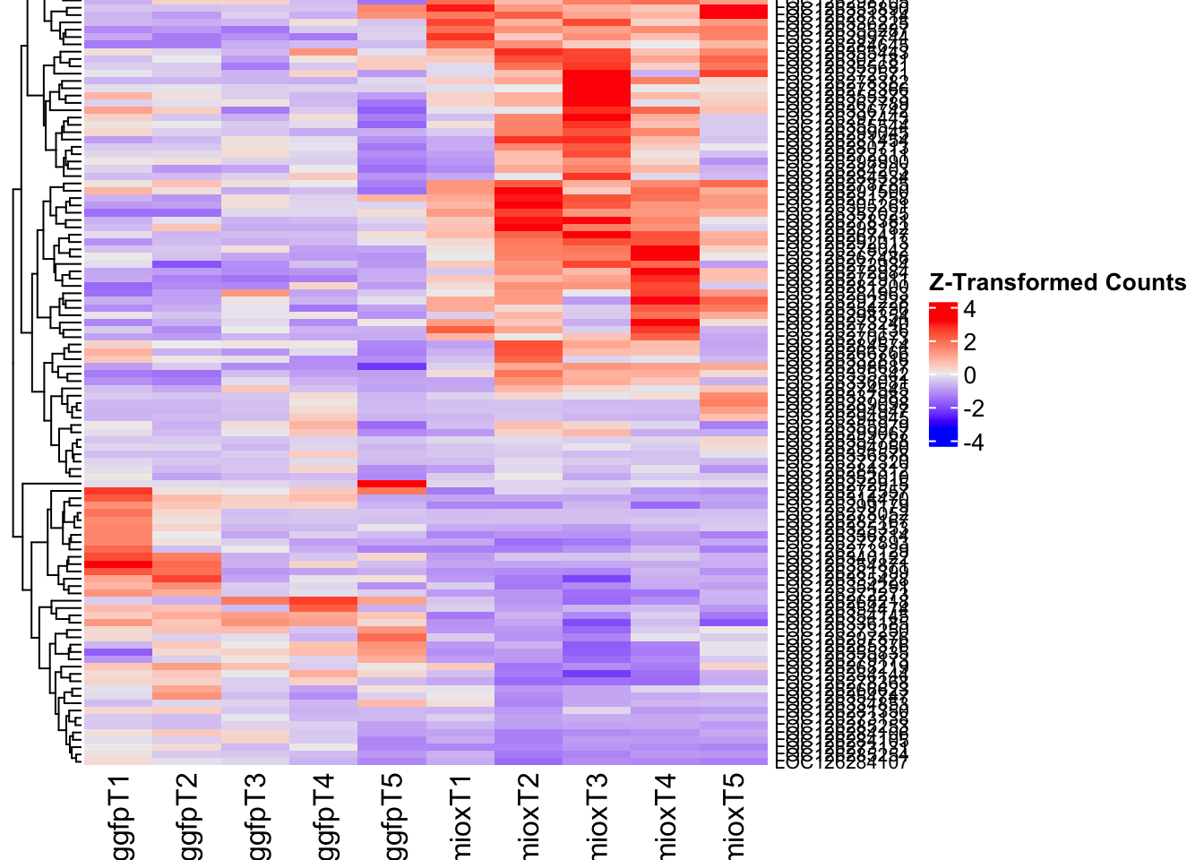
unch_plots$volcano; unch_plots$heatmap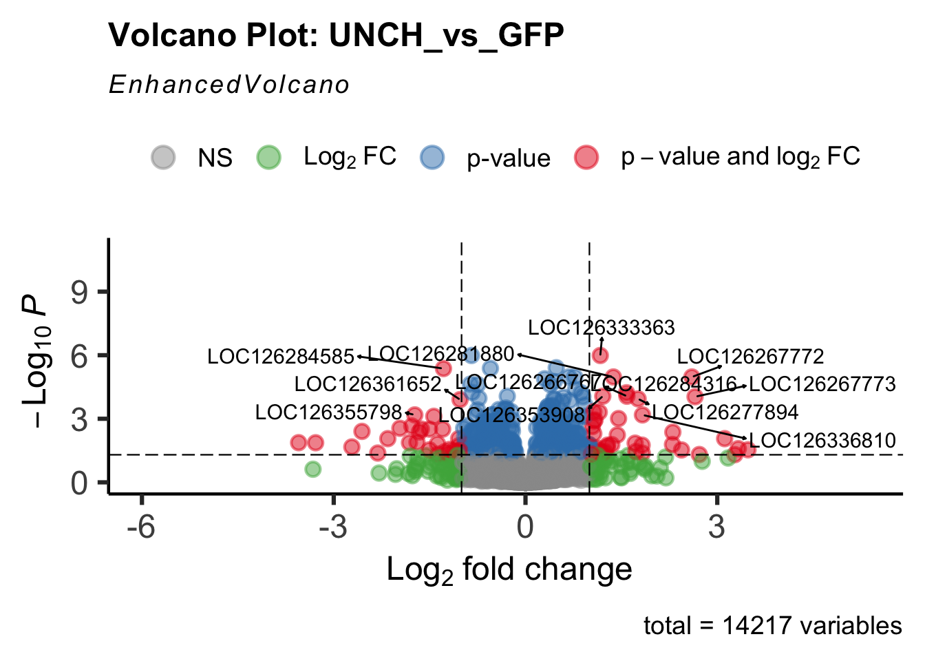
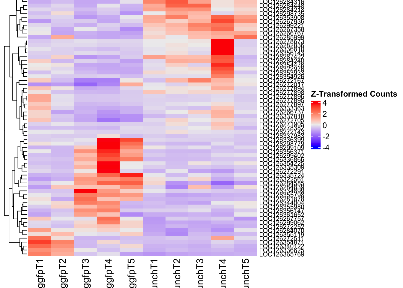
DEG tables
The following tables show the genes differentially expressed with at least an absolute log2fold change of > 1 considering thorax tissue only. Considering GFP as the reference state, upregulated genes in knockdown treatment in red and downregulated genes in knockdown treatment in blue. You can search for a gene of interest by writting a LOCID or description in the search bar or sort by column.
# Generate tables for each contrast
table_hex1 <- generate_deg_table(ddssva, "Gene_HEX1_vs_GFP", allspecies_df)
out of 14217 with nonzero total read count
adjusted p-value < 0.05
LFC > 0 (up) : 213, 1.5%
LFC < 0 (down) : 244, 1.7%
outliers [1] : 0, 0%
low counts [2] : 2757, 19%
(mean count < 30)
[1] see 'cooksCutoff' argument of ?results
[2] see 'independentFiltering' argument of ?resultsTotal DEGs p-value < 0.05 and absolute logFoldChange > 1: 40LFC > 1 (up) : 26 (65%)LFC < -1 (down) : 14 (35%)table_hex1$kable_tabletable_hex2 <- generate_deg_table(ddssva, "Gene_HEX2_vs_GFP", allspecies_df)
out of 14217 with nonzero total read count
adjusted p-value < 0.05
LFC > 0 (up) : 195, 1.4%
LFC < 0 (down) : 161, 1.1%
outliers [1] : 0, 0%
low counts [2] : 3308, 23%
(mean count < 42)
[1] see 'cooksCutoff' argument of ?results
[2] see 'independentFiltering' argument of ?resultsTotal DEGs p-value < 0.05 and absolute logFoldChange > 1: 16LFC > 1 (up) : 8 (50%)LFC < -1 (down) : 8 (50%)table_hex2$kable_tabletable_jhmt <- generate_deg_table(ddssva, "Gene_JHMT_vs_GFP", allspecies_df)
out of 14217 with nonzero total read count
adjusted p-value < 0.05
LFC > 0 (up) : 145, 1%
LFC < 0 (down) : 128, 0.9%
outliers [1] : 0, 0%
low counts [2] : 2481, 17%
(mean count < 26)
[1] see 'cooksCutoff' argument of ?results
[2] see 'independentFiltering' argument of ?resultsTotal DEGs p-value < 0.05 and absolute logFoldChange > 1: 52LFC > 1 (up) : 24 (46.15%)LFC < -1 (down) : 28 (53.85%)table_jhmt$kable_tabletable_miox <- generate_deg_table(ddssva, "Gene_MIOX_vs_GFP", allspecies_df)
out of 14217 with nonzero total read count
adjusted p-value < 0.05
LFC > 0 (up) : 475, 3.3%
LFC < 0 (down) : 403, 2.8%
outliers [1] : 0, 0%
low counts [2] : 827, 5.8%
(mean count < 10)
[1] see 'cooksCutoff' argument of ?results
[2] see 'independentFiltering' argument of ?resultsTotal DEGs p-value < 0.05 and absolute logFoldChange > 1: 111LFC > 1 (up) : 72 (64.86%)LFC < -1 (down) : 39 (35.14%)table_miox$kable_tabletable_unch <- generate_deg_table(ddssva, "Gene_UNCH_vs_GFP", allspecies_df)
out of 14217 with nonzero total read count
adjusted p-value < 0.05
LFC > 0 (up) : 287, 2%
LFC < 0 (down) : 278, 2%
outliers [1] : 0, 0%
low counts [2] : 3032, 21%
(mean count < 35)
[1] see 'cooksCutoff' argument of ?results
[2] see 'independentFiltering' argument of ?resultsTotal DEGs p-value < 0.05 and absolute logFoldChange > 1: 69LFC > 1 (up) : 39 (56.52%)LFC < -1 (down) : 30 (43.48%)table_unch$kable_tableSummary and Overlap
# Summarize DEGs for all contrasts
deg_summary <- bind_rows(
summarize_deg_counts(table_hex1, "HEX1 vs GFP"),
summarize_deg_counts(table_hex2, "HEX2 vs GFP"),
summarize_deg_counts(table_jhmt, "JHMT vs GFP"),
summarize_deg_counts(table_miox, "MIOX vs GFP"),
summarize_deg_counts(table_unch, "UNCH vs GFP")
)
# Display table using kable with styling
deg_summary %>%
kable("html", escape = FALSE, col.names = gsub("_", " ", names(.))) %>%
kable_styling("striped", full_width = TRUE) %>%
column_spec(2, color = "red", bold = TRUE) %>% # Upregulated in red
column_spec(3, color = "blue", bold = TRUE) %>% # Downregulated in blue
add_header_above(c("Summary of DEGs" = 3)) %>%
row_spec(0, bold = TRUE)| Contrast | Upregulated | Downregulated |
|---|---|---|
| HEX1 vs GFP | 26 | 12 |
| HEX2 vs GFP | 7 | 8 |
| JHMT vs GFP | 22 | 26 |
| MIOX vs GFP | 68 | 35 |
| UNCH vs GFP | 35 | 28 |
# Define the list of RNAi contrasts
contrast_list <- c("HEX1_vs_GFP", "HEX2_vs_GFP", "JHMT_vs_GFP",
"MIOX_vs_GFP", "UNCH_vs_GFP")
# Initialize empty lists for storing Head-specific DEGs for each contrast
venn_data_up <- list()
venn_data_down <- list()
venn_data_all <- list()
# Function to load Head-specific DEGs for a given set of contrasts
load_deg_contrasts_head <- function(contrast_list) {
degs_up <- list()
degs_down <- list()
degs_all <- list()
for (contrast in contrast_list) {
deg_file <- file.path(workDir, "DEG_results/RNAi/Thorax_no_rRNA/", contrast, paste0("DEG_sigresults_", contrast, ".csv"))
if (!file.exists(deg_file)) {
message(paste("File missing for contrast:", contrast))
next # Skip if the file doesn't exist
}
deg_data <- read.csv(deg_file, stringsAsFactors = FALSE)
# Convert row names to a column if necessary
if ("X" %in% colnames(deg_data)) {
colnames(deg_data)[colnames(deg_data) == "X"] <- "GeneID"
}
# Check if data is empty
if (nrow(deg_data) == 0) {
message(paste("No data for contrast:", contrast))
next
}
# Select significant DEGs (Up, Down, All)
degs_up[[contrast]] <- deg_data %>%
filter(padj < 0.05 & log2FoldChange >= 1) %>%
pull(GeneID) # Extract GeneID column
degs_down[[contrast]] <- deg_data %>%
filter(padj < 0.05 & log2FoldChange <= -1) %>%
pull(GeneID) # Extract GeneID column
degs_all[[contrast]] <- deg_data %>%
filter(padj < 0.05 & abs(log2FoldChange) >= 1) %>%
pull(GeneID) # Extract GeneID column
}
return(list(up = degs_up, down = degs_down, all = degs_all))
}
# Load DEG data for the defined contrasts (Head tissue only)
venn_data_contrasts <- load_deg_contrasts_head(contrast_list)
# Prepare the data for the Venn diagrams
venn_data_up <- venn_data_contrasts$up
venn_data_down <- venn_data_contrasts$down
venn_data_all <- venn_data_contrasts$all
# Function to display Venn diagram and corresponding datatable
display_venn_with_datatable <- function(venn_data, title, allspecies_df) {
# Calculate the overlapping genes
overlap_genes <- Reduce(intersect, venn_data)
# Create a data frame for the overlapping genes
overlap_df <- data.frame(GeneID = overlap_genes)
# Merge to get species information
meta_brock_df <- merge(overlap_df, allspecies_df, by = "GeneID", all.x = TRUE)
# Generate the Venn diagram
venn_plot <- venn.diagram(
x = venn_data,
category.names = contrast_list,
filename = NULL,
output = TRUE,
fill = c("orange", "red", "blue", "purple", "green"), # Adjust colors for contrasts
alpha = 0.5,
cex = 2,
cat.cex = 0,
main = title,
main.cex = 1.2
)
# Clear the plotting area before drawing
grid.newpage()
grid.draw(venn_plot)
# Create a custom legend
legend_labels <- contrast_list
legend_colors <- c("orange", "red", "blue", "purple", "green")
# Positioning the legend
legend_x <- unit(0.85, "npc") # Adjust x position
legend_y <- unit(0.2, "npc") # Adjust y position
# Draw the legend
for (i in 1:length(legend_labels)) {
grid.rect(x = legend_x, y = legend_y - unit((i - 1) * 0.05, "npc"),
width = unit(0.02, "npc"), height = unit(0.02, "npc"),
gp = gpar(fill = legend_colors[i], col = NA))
grid.text(label = legend_labels[i], x = legend_x + unit(0.05, "npc"),
y = legend_y - unit((i - 1) * 0.05, "npc"),
just = "left", gp = gpar(cex = 0.8))
}
# Display the merged overlapping genes table with datatable
datatable(meta_brock_df, options = list(
pageLength = 10,
scrollX = TRUE,
autoWidth = TRUE,
searchHighlight = TRUE
),
rownames = FALSE,
escape = FALSE
) %>%
formatStyle(
'Species', target = 'cell',
fontStyle = 'italic'
) %>%
formatStyle(
columns = names(meta_brock_df),
target = 'row',
color = styleEqual(c("red", "blue", "black"), c("red", "blue", "black")),
fontWeight = styleEqual(c("bold", "normal"), c("bold", "normal")),
backgroundColor = styleEqual(c("red", "blue", "black"), c("white", "white", "white"))
)
}
# Display the Venn diagram and datatable for **Head Upregulated DEGs** across contrasts
display_venn_with_datatable(venn_data_up, "Venn Diagram of Head Upregulated DEGs - RNAi Contrasts", allspecies_df)
| Version | Author | Date |
|---|---|---|
| b540a1e | Maeva TECHER | 2025-02-27 |
# Display the Venn diagram and datatable for **Head Downregulated DEGs** across contrasts
display_venn_with_datatable(venn_data_down, "Venn Diagram of Head Downregulated DEGs - RNAi Contrasts", allspecies_df)
| Version | Author | Date |
|---|---|---|
| b540a1e | Maeva TECHER | 2025-02-27 |
# Display the Venn diagram and datatable for **All Significant DEGs in Head Tissue**
display_venn_with_datatable(venn_data_all, "Venn Diagram of All Significant DEGs in Head Tissue - RNAi Contrasts", allspecies_df)
| Version | Author | Date |
|---|---|---|
| b540a1e | Maeva TECHER | 2025-02-27 |
GO and KEGG enrichment
#enrich_data(hex1, "Hex1_vs_GFP", hex1_samples)
#enrich_data(hex2, "Hex2_vs_GFP", hex2_samples)
#enrich_data(jhmt, "JHMT_vs_GFP", jhmt_samples)
#enrich_data(miox, "MIOX_vs_GFP", miox_samples)
#enrich_data(unch, "UNCH_vs_GFP", unch_samples)5. Comparison between injected and non-injected crowded
All genes included
All tissue together
Minor changes here are made compared to the DESeq2
results regarding the importation of samples to transform into a
matrix.
Sample names are structured as follow: {Sg}{gene}{#} {Sg} = Schistocerca gregaria {gene} = gene abbreviation gfp, hex1, hex2, jhmt, miox and unch H/T{#} = biological replicate
saveDir <- paste0(workDir,"/DEG_results/RNAi/All_control")
dir.create(saveDir)
### Prepare Sample CSV file #####
samples <- read.delim(file.path(workDir, "list/RNAi/All_RNAi_noninjectedsample_list.csv"), sep = ",", row.names = 1, header = TRUE)
files <- file.path(workDir, "readcounts/RNAi/", samples$Tissue, samples$Filename)
names(files) <- row.names(samples)
if (all(file.exists(files))) {
message("All the files exist!")
} else {
warning("Some files are missing!")
}All the files exist!### **Standardized Count Matrix Creation**
# Extract all gene lists first
gene_lists <- map(files, function(sample) {
fread(sample, sep = "\t", header = FALSE)[, 1] # Extract Gene IDs (column 1)
})
# Get a unique set of all gene IDs across all samples
all_genes <- unique(unlist(gene_lists))
# Create a named list to store count data with standardized rows
cts_list <- map(files, function(sample) {
data_count <- fread(sample, sep = "\t", header = FALSE)
col_name <- gsub("_counts.txt", "", basename(sample)) # Clean sample name
# Convert to data frame with correct column names
data_count <- setNames(data.frame(data_count[, 1:2]), c("GeneID", col_name))
# Ensure all gene IDs are present (fill missing values with 0)
data_count <- full_join(data.frame(GeneID = all_genes), data_count, by = "GeneID") %>%
mutate(across(where(is.numeric), ~ replace_na(., 0))) # Fill NA with 0
return(data_count)
})
# Merge all samples based on GeneID
cts <- reduce(cts_list, full_join, by = "GeneID")
# Convert to matrix for DESeq2
cts_matrix <- as.matrix(cts[, -1]) # Remove GeneID column for count matrix
rownames(cts_matrix) <- cts$GeneID # Set GeneID as rownames
rm(cts_list) # Free memoryWhile for bulk RNAseq on head and thorax for all species, the DEGs model was made between isolated and crowded individuals (with isolated as the reference state), here, the DEG analysis will be carried between GFP knock-down nymphs (as reference state) vs Hexamerins / Juvenile Hormones / Inositol / Uncharacterized proteins.
### Build DESeq2 Object
dds <- DESeqDataSetFromMatrix(countData = cts_matrix,
colData = samples,
design = ~ Gene)
dds$Gene <- relevel(dds$Gene, ref = "CONTROL")
smallestGroupSize <- 5
keep <- rowSums(counts(dds) >= 10) >= smallestGroupSize
dds <- dds[keep,]
dds <- DESeq(dds)Normalization and PCA
# Plot PCA and investigate quality metrics
vsd <- vst(dds, blind = TRUE)
# Perform PCA
pca_data <- plotPCA(vsd, intgroup = c("Tissue", "Gene"), returnData = TRUE)
# Define colors for genes (slightly transparent) and shapes for tissues
gene_colors <- scale_color_manual(values = alpha(brewer.pal(n = length(unique(pca_data$Gene)), name = "Set1"), 0.8)) # Points are transparent
tissue_shapes <- scale_shape_manual(values = seq(15, 15 + length(unique(pca_data$Tissue))))
# **PCA without labels**
p_pca_nolabel <- ggplot(pca_data, aes(x = PC1, y = PC2, color = Gene, shape = Tissue)) +
geom_point(size = 4) +
gene_colors +
tissue_shapes +
theme_bw() +
theme(legend.title = element_blank(),
legend.text = element_text(face = "bold", size = 14),
axis.text = element_text(size = 12),
axis.title = element_text(size = 14)) +
ggtitle("PCA of All Tissues (No Labels)", subtitle = "Tissues differentiated by shape, Genes by color")
# Save PCA without labels
ggsave(paste0(saveDir, "/PCA_Tissue_Gene_NoLabel.png"), plot = p_pca_nolabel, width = 10, height = 10, dpi = 600, device = "png")
# **PCA with labels**
p_pca_label <- ggplot(pca_data, aes(x = PC1, y = PC2, color = Gene, shape = Tissue)) +
geom_point(size = 4) +
geom_text_repel(aes(label = name), size = 4, color = "black", max.overlaps = 20) + # Labels are fully visible
gene_colors +
tissue_shapes +
theme_bw() +
theme(legend.title = element_blank(),
legend.text = element_text(face = "bold", size = 14),
axis.text = element_text(size = 12),
axis.title = element_text(size = 14)) +
ggtitle("PCA of All Tissues (With Labels)", subtitle = "Tissues differentiated by shape, Genes by color")
# Save PCA with labels
ggsave(paste0(saveDir, "/PCA_Tissue_Gene_Label.png"), plot = p_pca_label, width = 10, height = 10, dpi = 600, device = "png")
# **Return plots for knitr/RMarkdown**
list(NoLabel = p_pca_nolabel, WithLabel = p_pca_label)$NoLabel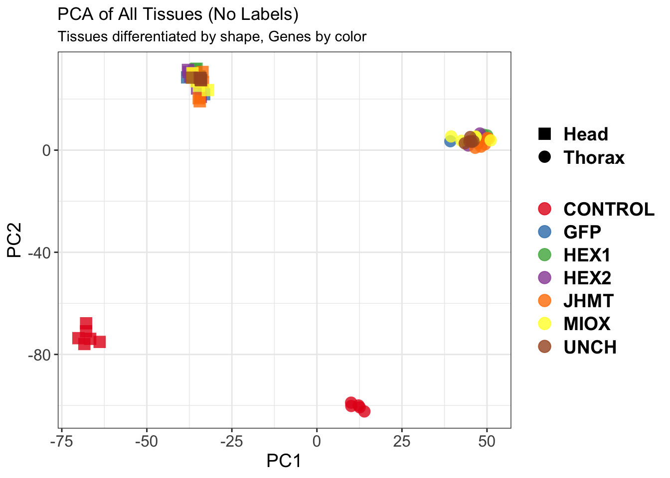
| Version | Author | Date |
|---|---|---|
| b540a1e | Maeva TECHER | 2025-02-27 |
$WithLabel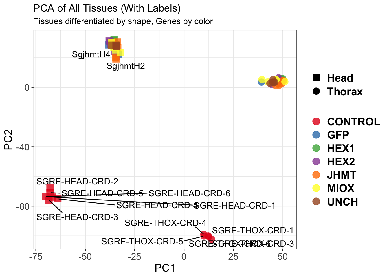
| Version | Author | Date |
|---|---|---|
| b540a1e | Maeva TECHER | 2025-02-27 |
The PCA plot shows clear distinction between tissue types, while gene silencing has a large variation within each tissue, and presents no distinct clear groupings for a single gene.
SVA
### SVA analysis to control for technical variation
dat <- counts(dds, normalized = TRUE)
idx <- rowMeans(dat) > 1
dat <- dat[idx, ]
mod <- model.matrix(~ Gene, colData(dds))
mod0 <- model.matrix(~ 1, colData(dds))
svseq <- svaseq(dat, mod, mod0)Number of significant surrogate variables is: 4
Iteration (out of 5 ):1 2 3 4 5 sva_plots <- create_sva_plots(svseq, dds, saveDir, intgroup = c("Tissue", "Gene"), max_sv = 4)
# Show stripcharts in the report
sva_plots$Stripcharts[[1]] # Show first stripchart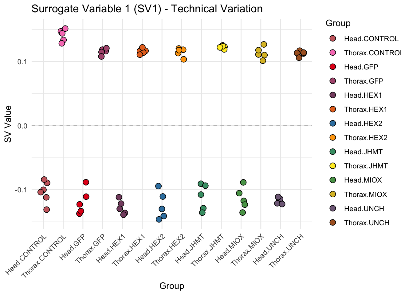
| Version | Author | Date |
|---|---|---|
| b540a1e | Maeva TECHER | 2025-02-27 |
sva_plots$Stripcharts[[2]] # Show second stripchart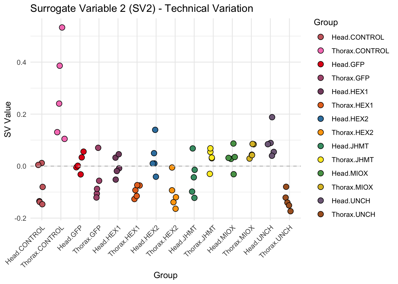
| Version | Author | Date |
|---|---|---|
| b540a1e | Maeva TECHER | 2025-02-27 |
sva_plots$Stripcharts[[3]] # Show third stripchart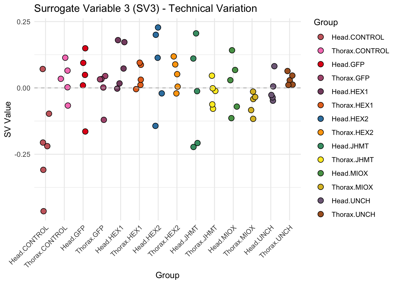
| Version | Author | Date |
|---|---|---|
| b540a1e | Maeva TECHER | 2025-02-27 |
sva_plots$Stripcharts[[4]] 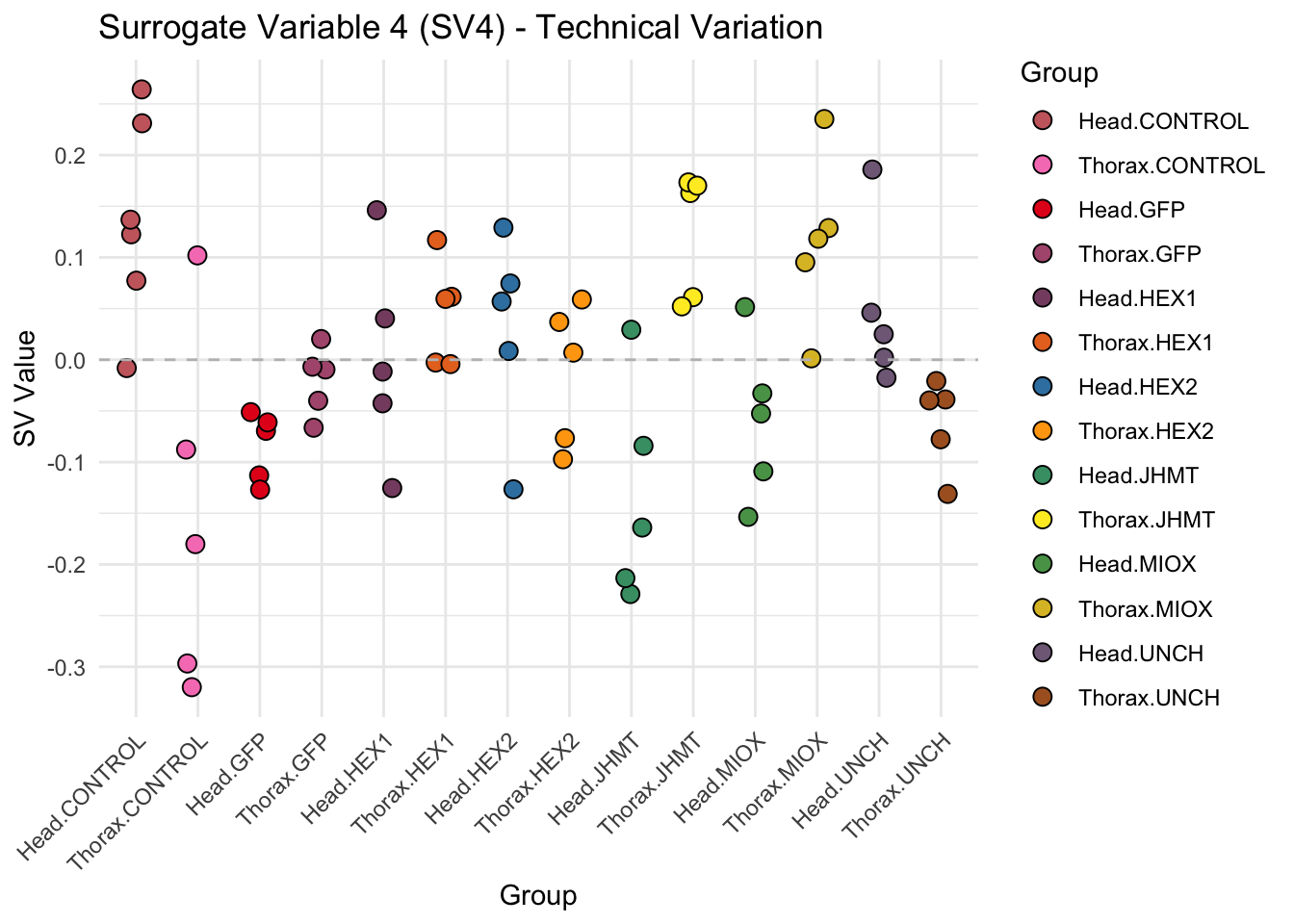
| Version | Author | Date |
|---|---|---|
| b540a1e | Maeva TECHER | 2025-02-27 |
# Show scatter plots in the report
sva_plots$ScatterPlots[["1_2"]] # Show SV1 vs SV2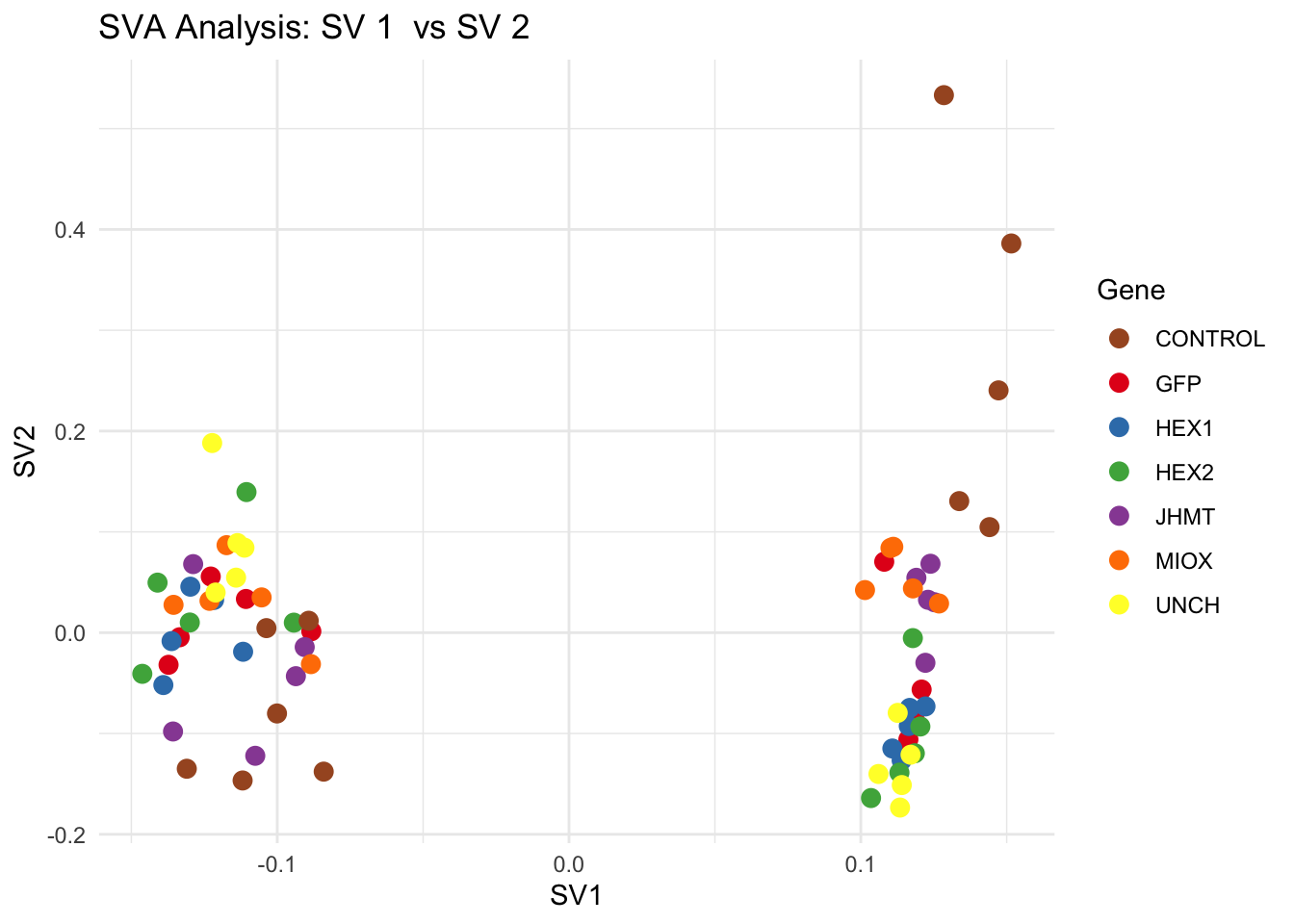
| Version | Author | Date |
|---|---|---|
| b540a1e | Maeva TECHER | 2025-02-27 |
sva_plots$ScatterPlots[["1_3"]] # Show SV1 vs SV3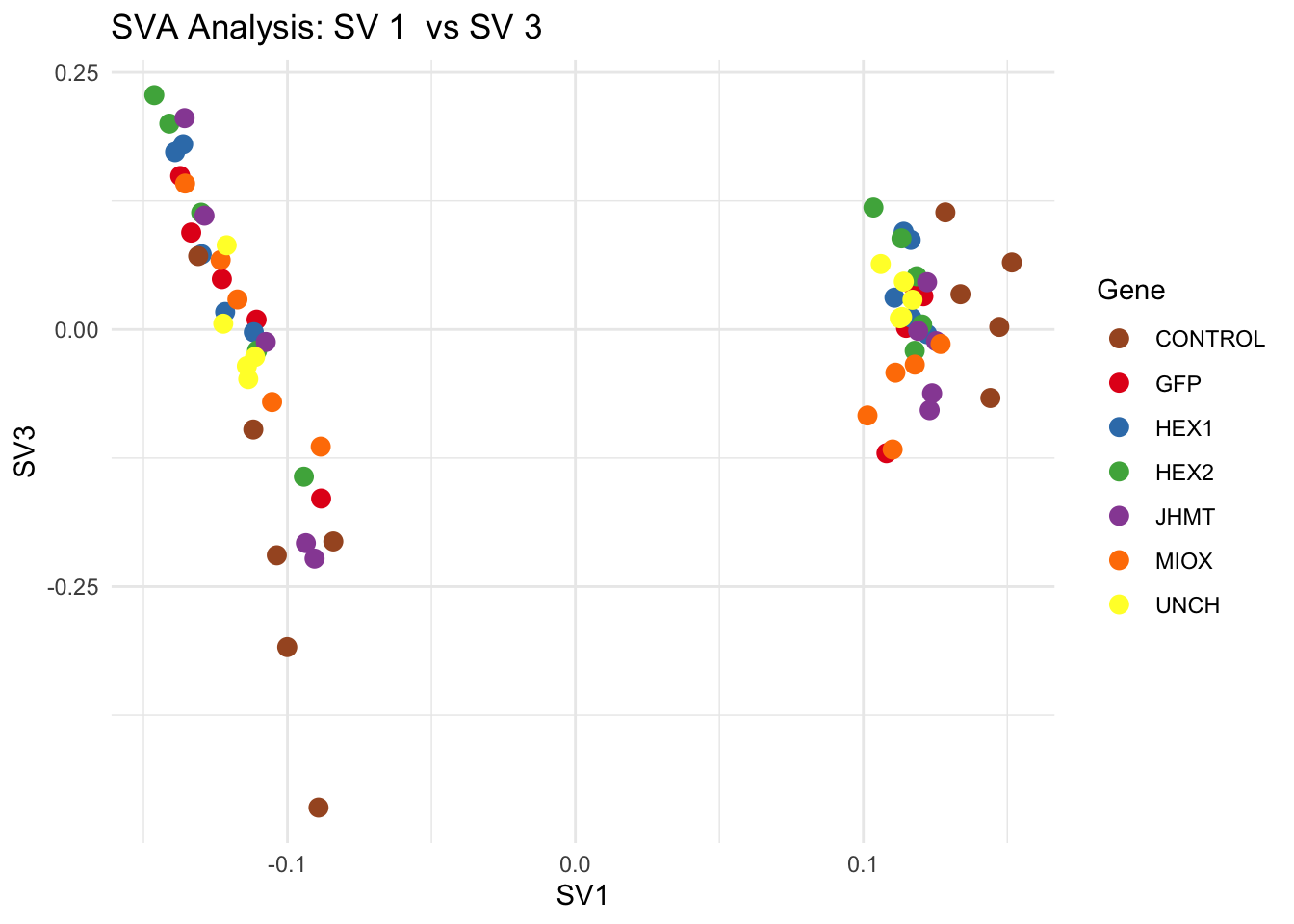
| Version | Author | Date |
|---|---|---|
| b540a1e | Maeva TECHER | 2025-02-27 |
sva_plots$ScatterPlots[["2_3"]] # Show SV2 vs SV3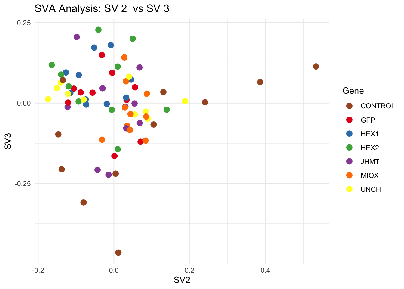
| Version | Author | Date |
|---|---|---|
| b540a1e | Maeva TECHER | 2025-02-27 |
SV1 is clearly showing an effect of tissue. We rerun the
DESeq2 model but this time including the surrogate variable
SV2 and SV3 as a covariates only, as we know that the modeled variation
is more likely explained by tissue and gene variation rather than batch
effects.
ddssva <- dds
ddssva$SV2 <- svseq$sv[,2]
ddssva$SV3 <- svseq$sv[,3]
ddssva$SV4 <- svseq$sv[,4]
design(ddssva) <- ~ SV2 + SV3 + SV4 + Gene
ddssva$Gene <- relevel(ddssva$Gene, ref = "CONTROL")
smallestGroupSize <- 5
keep <- rowSums(counts(ddssva) >= 10) >= smallestGroupSize
ddssva <- ddssva[keep,]
ddssva <- DESeq(ddssva)
ddssva <- ddssva[which(mcols(ddssva)$betaConv),] # remove non converging rows
### Extract results
message("Available contrasts are: ", paste(resultsNames(ddssva), collapse = ", "))
hex1 <- results(ddssva, contrast = c("Gene", "HEX1", "CONTROL"), alpha = 0.05)
hex2 <- results(ddssva, contrast = c("Gene", "HEX2", "CONTROL"), alpha = 0.05)
jhmt <- results(ddssva, contrast = c("Gene", "JHMT", "CONTROL"), alpha = 0.05)
miox <- results(ddssva, contrast = c("Gene", "MIOX", "CONTROL"), alpha = 0.05)
unch <- results(ddssva, contrast = c("Gene", "UNCH", "CONTROL"), alpha = 0.05)
gfp <- results(ddssva, contrast = c("Gene", "GFP", "CONTROL"), alpha = 0.05)Volcano plots and Heatmaps
# Define contrast_sets
hex1_samples <- c("SGRE-HEAD-CRD-1","SGRE-HEAD-CRD-2","SGRE-HEAD-CRD-3","SGRE-HEAD-CRD-4","SGRE-HEAD-CRD-5",
"SGRE-HEAD-CRD-6","SggfpH1","SggfpH2","SggfpH3","SggfpH4","SggfpH5",
"Sghex1H1","Sghex1H2","Sghex1H3","Sghex1H4","Sghex1H5",
"SGRE-THOX-CRD-1","SGRE-THOX-CRD-3","SGRE-THOX-CRD-4","SGRE-THOX-CRD-5",
"SGRE-THOX-CRD-6","SggfpT1","SggfpT2","SggfpT3","SggfpT4","SggfpT5",
"Sghex1T1","Sghex1T2","Sghex1T3","Sghex1T4","Sghex1T5")
hex2_samples <- c("SGRE-HEAD-CRD-1","SGRE-HEAD-CRD-2","SGRE-HEAD-CRD-3","SGRE-HEAD-CRD-4","SGRE-HEAD-CRD-5",
"SGRE-HEAD-CRD-6","SggfpH1","SggfpH2","SggfpH3","SggfpH4","SggfpH5",
"Sghex2H1","Sghex2H2","Sghex2H3","Sghex2H4","Sghex2H5",
"SGRE-THOX-CRD-1","SGRE-THOX-CRD-3","SGRE-THOX-CRD-4","SGRE-THOX-CRD-5",
"SGRE-THOX-CRD-6","SggfpT1","SggfpT2","SggfpT3","SggfpT4","SggfpT5",
"Sghex2T1","Sghex2T2","Sghex2T3","Sghex2T4","Sghex2T5")
jhmt_samples <- c("SGRE-HEAD-CRD-1","SGRE-HEAD-CRD-2","SGRE-HEAD-CRD-3","SGRE-HEAD-CRD-4","SGRE-HEAD-CRD-5",
"SGRE-HEAD-CRD-6","SggfpH1","SggfpH2","SggfpH3","SggfpH4","SggfpH5",
"SgjhmtH1","SgjhmtH2","SgjhmtH3","SgjhmtH4","SgjhmtH5",
"SGRE-THOX-CRD-1","SGRE-THOX-CRD-3","SGRE-THOX-CRD-4","SGRE-THOX-CRD-5",
"SGRE-THOX-CRD-6","SggfpT1","SggfpT2","SggfpT3","SggfpT4","SggfpT5",
"SgjhmtT1","SgjhmtT2","SgjhmtT3","SgjhmtT4","SgjhmtT5")
miox_samples <- c("SGRE-HEAD-CRD-1","SGRE-HEAD-CRD-2","SGRE-HEAD-CRD-3","SGRE-HEAD-CRD-4","SGRE-HEAD-CRD-5",
"SGRE-HEAD-CRD-6","SggfpH1","SggfpH2","SggfpH3","SggfpH4","SggfpH5",
"SgmioxH1","SgmioxH2","SgmioxH3","SgmioxH4","SgmioxH5",
"SGRE-THOX-CRD-1","SGRE-THOX-CRD-3","SGRE-THOX-CRD-4","SGRE-THOX-CRD-5",
"SGRE-THOX-CRD-6","SggfpT1","SggfpT2","SggfpT3","SggfpT4","SggfpT5",
"SgmioxT1","SgmioxT2","SgmioxT3","SgmioxT4","SgmioxT5")
unch_samples <- c("SGRE-HEAD-CRD-1","SGRE-HEAD-CRD-2","SGRE-HEAD-CRD-3","SGRE-HEAD-CRD-4","SGRE-HEAD-CRD-5",
"SGRE-HEAD-CRD-6","SggfpH1","SggfpH2","SggfpH3","SggfpH4","SggfpH5",
"SgunchH1","SgunchH2","SgunchH3","SgunchH4","SgunchH5",
"SGRE-THOX-CRD-1","SGRE-THOX-CRD-3","SGRE-THOX-CRD-4","SGRE-THOX-CRD-5",
"SGRE-THOX-CRD-6","SggfpT1","SggfpT2","SggfpT3","SggfpT4","SggfpT5",
"SgunchT1","SgunchT2","SgunchT3","SgunchT4","SgunchT5")
gfp_samples <- c("SGRE-HEAD-CRD-1","SGRE-HEAD-CRD-2","SGRE-HEAD-CRD-3","SGRE-HEAD-CRD-4","SGRE-HEAD-CRD-5",
"SGRE-HEAD-CRD-6","SggfpH1","SggfpH2","SggfpH3","SggfpH4","SggfpH5", "SGRE-THOX-CRD-1","SGRE-THOX-CRD-3","SGRE-THOX-CRD-4","SGRE-THOX-CRD-5",
"SGRE-THOX-CRD-6", "SggfpT1","SggfpT2","SggfpT3","SggfpT4","SggfpT5")
# Run full analysis
hex1_plots <- visualize_data_nopng(hex1, "HEX1_vs_CONTROL", hex1_samples)
hex2_plots <- visualize_data_nopng(hex2, "HEX2_vs_CONTROL", hex2_samples)
jhmt_plots <- visualize_data_nopng(jhmt, "JHMT_vs_CONTROL", jhmt_samples)
miox_plots <- visualize_data_nopng(miox, "MIOX_vs_CONTROL", miox_samples)
unch_plots <- visualize_data_nopng(unch, "UNCH_vs_CONTROL", unch_samples)
gfp_plots <- visualize_data_nopng(gfp, "GFP_vs_CONTROL", gfp_samples)
hex1_plots$volcano; hex1_plots$heatmap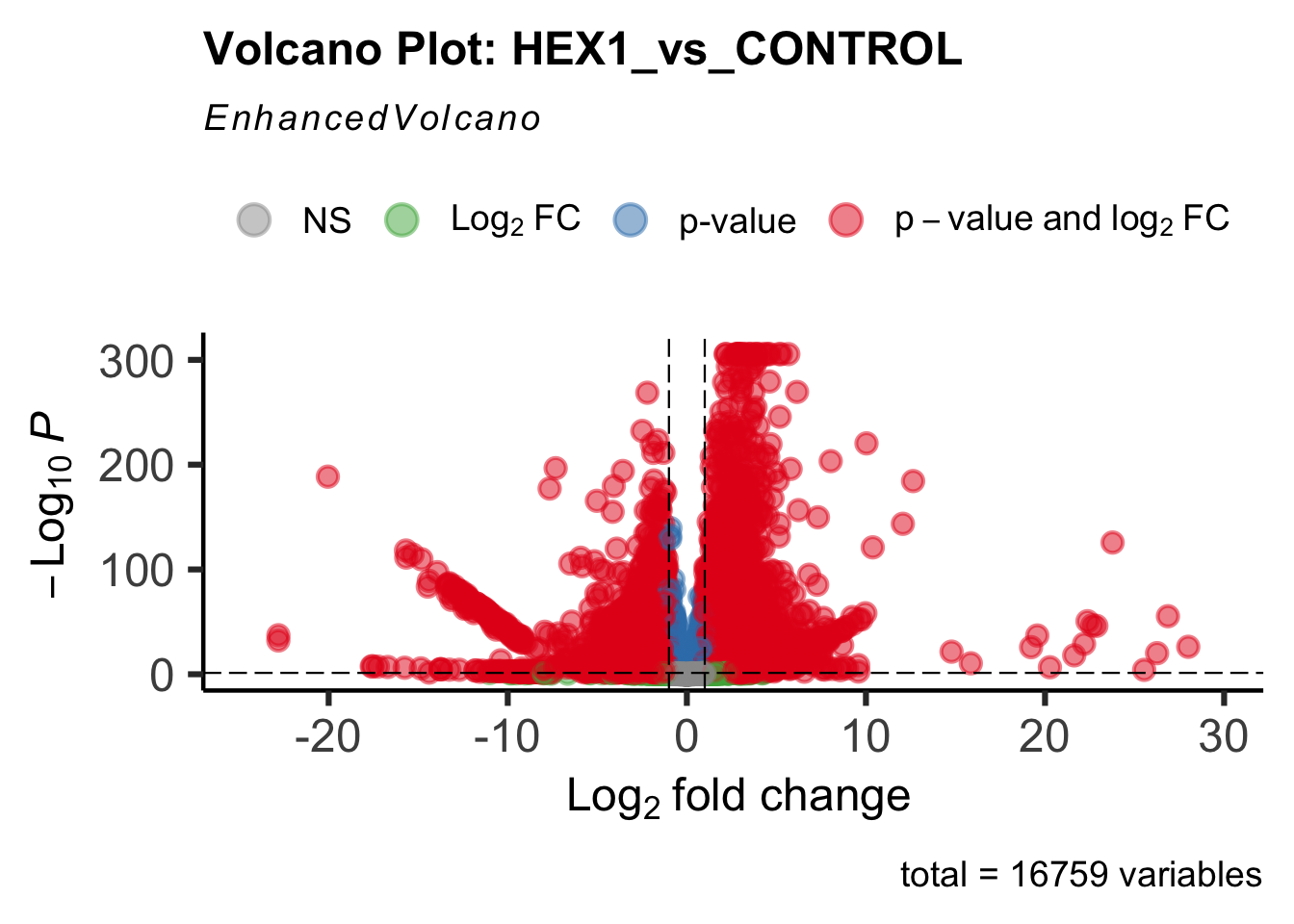
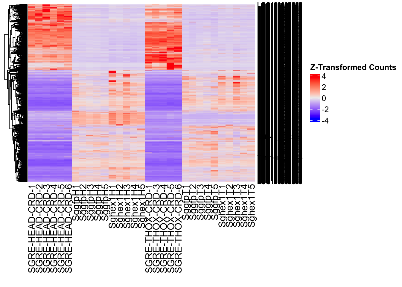
| Version | Author | Date |
|---|---|---|
| b540a1e | Maeva TECHER | 2025-02-27 |
hex2_plots$volcano; hex2_plots$heatmap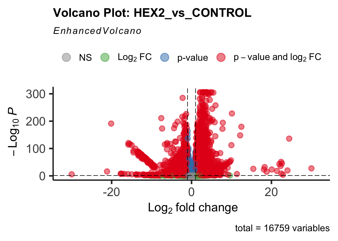
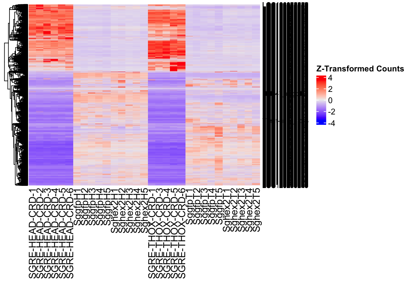
| Version | Author | Date |
|---|---|---|
| b540a1e | Maeva TECHER | 2025-02-27 |
jhmt_plots$volcano; jhmt_plots$heatmap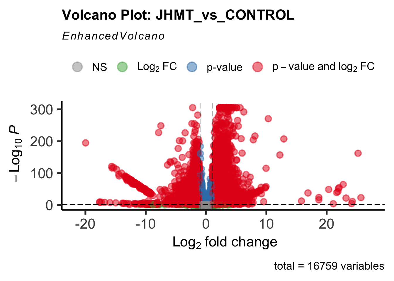
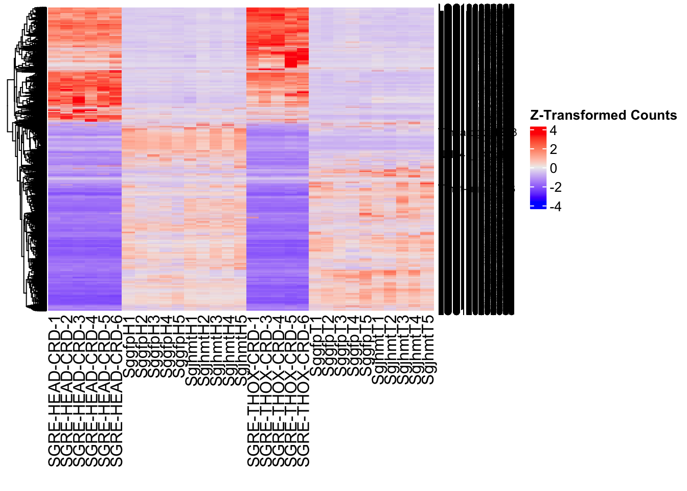
| Version | Author | Date |
|---|---|---|
| b540a1e | Maeva TECHER | 2025-02-27 |
miox_plots$volcano; miox_plots$heatmap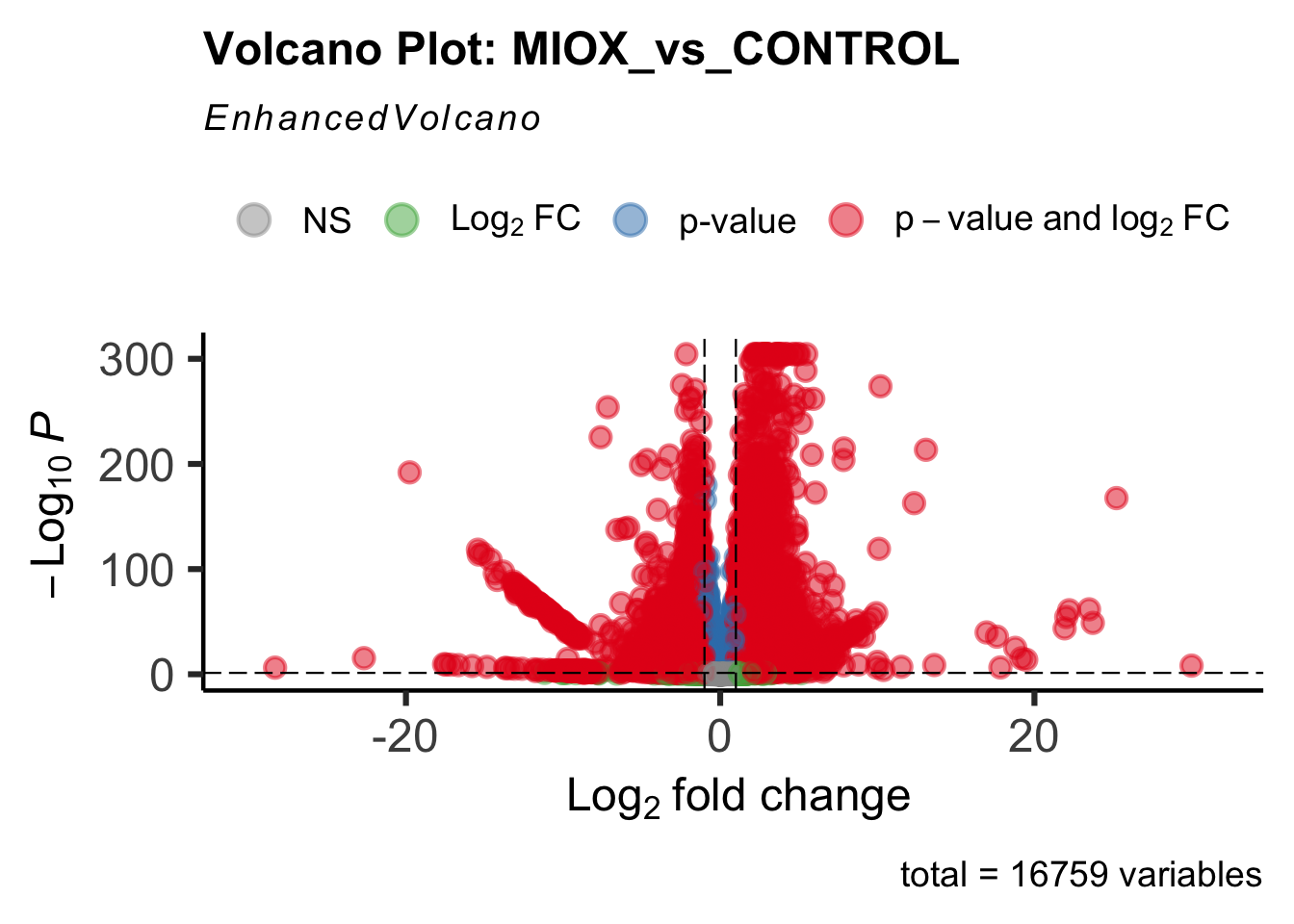
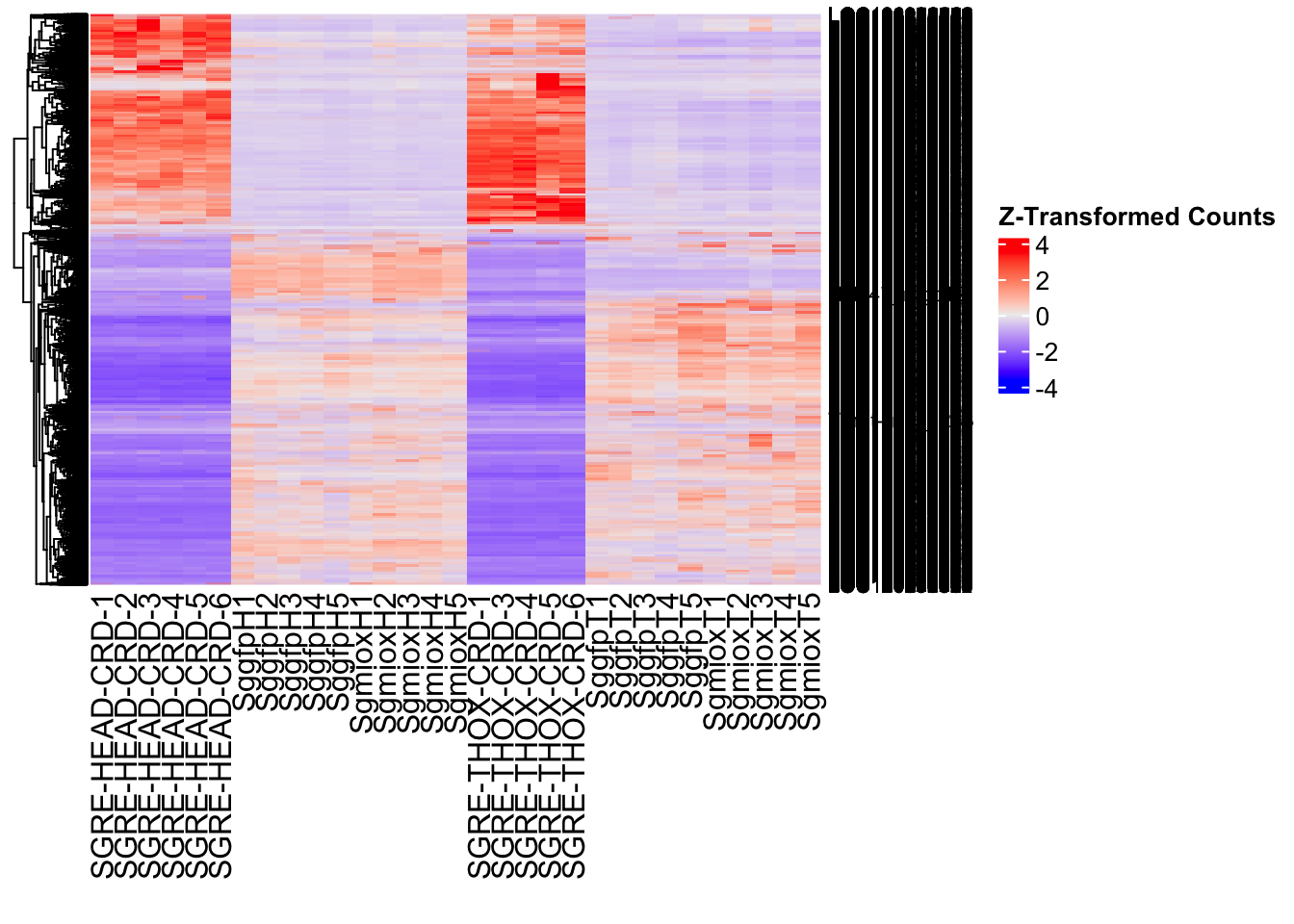
| Version | Author | Date |
|---|---|---|
| b540a1e | Maeva TECHER | 2025-02-27 |
unch_plots$volcano; unch_plots$heatmap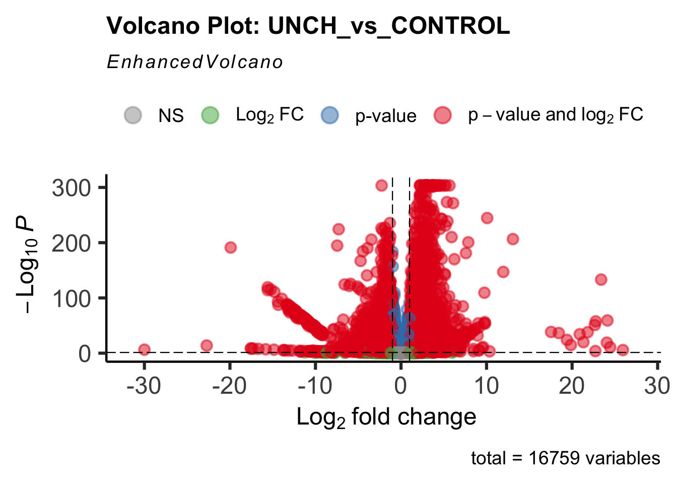
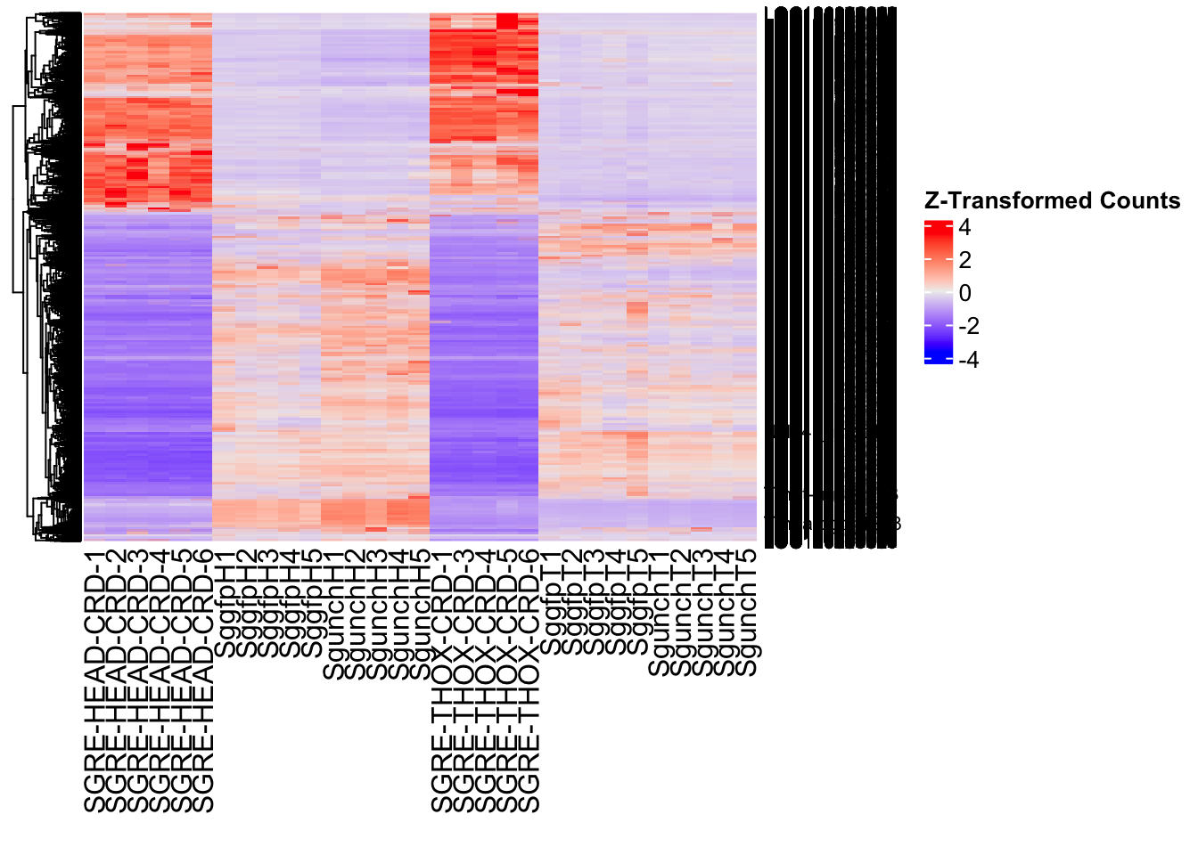
| Version | Author | Date |
|---|---|---|
| b540a1e | Maeva TECHER | 2025-02-27 |
gfp_plots$volcano; gfp_plots$heatmap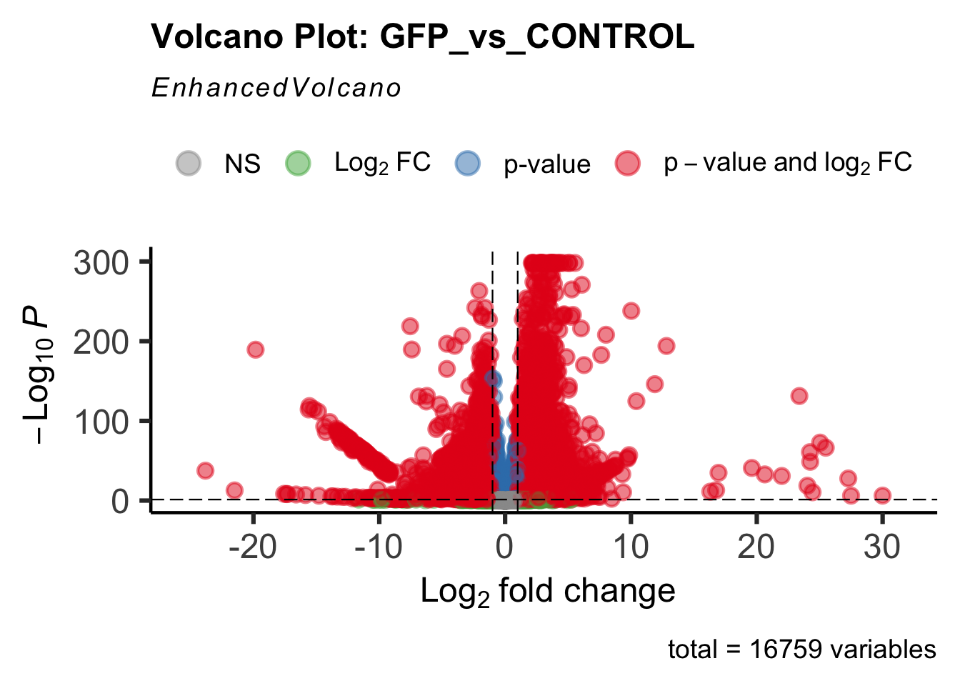
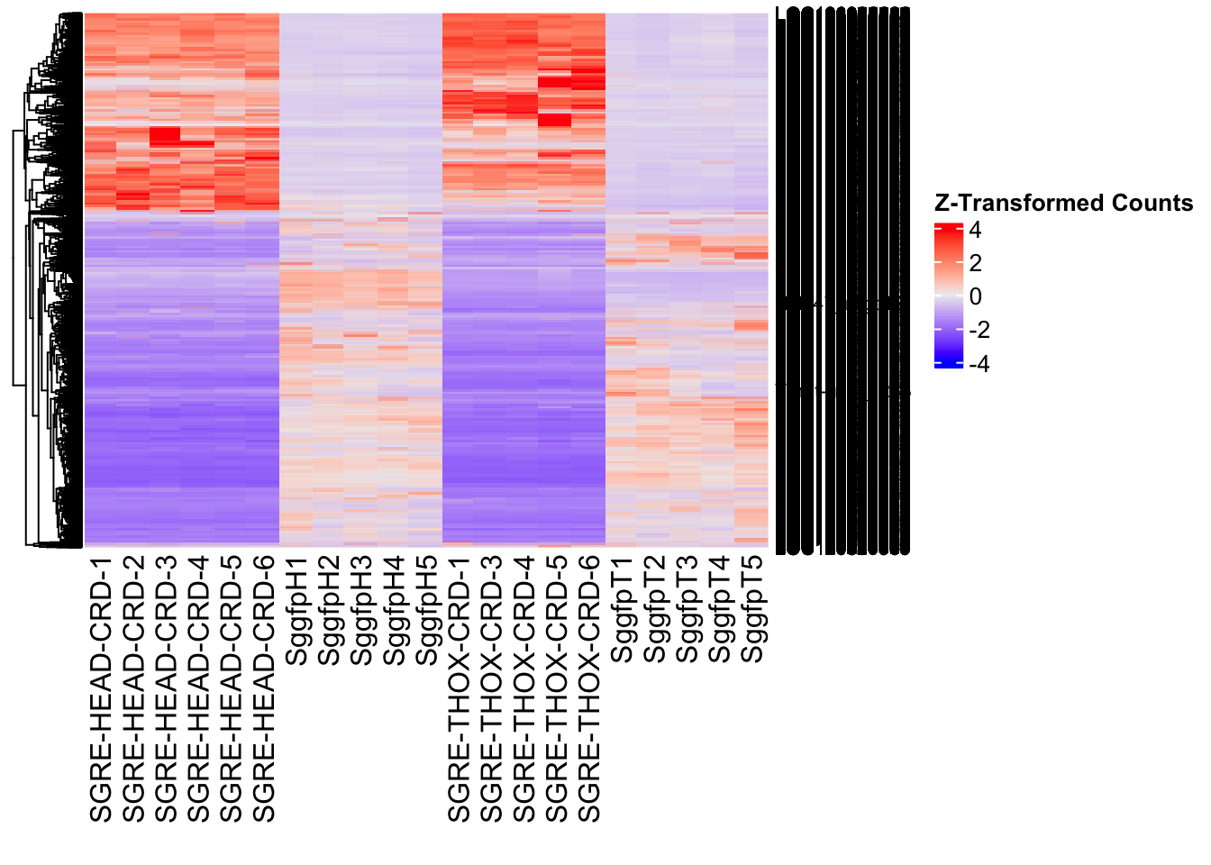
DEG tables
The following tables show the genes differentially expressed with at least an absolute log2fold change of > 1 considering all tissues together. Considering GFP as the reference state, upregulated genes in knockdown treatment in red and downregulated genes in knockdown treatment in blue. You can search for a gene of interest by writting a LOCID or description in the search bar or sort by column.
# Generate tables for each contrast
table_hex1 <- generate_deg_table(ddssva, "Gene_HEX1_vs_CONTROL", allspecies_df)
out of 16759 with nonzero total read count
adjusted p-value < 0.05
LFC > 0 (up) : 8238, 49%
LFC < 0 (down) : 5539, 33%
outliers [1] : 0, 0%
low counts [2] : 0, 0%
(mean count < 1)
[1] see 'cooksCutoff' argument of ?results
[2] see 'independentFiltering' argument of ?resultsTotal DEGs p-value < 0.05 and absolute logFoldChange > 1: 10376LFC > 1 (up) : 6513 (62.77%)LFC < -1 (down) : 3863 (37.23%)table_hex1$kable_tabletable_hex2 <- generate_deg_table(ddssva, "Gene_HEX2_vs_CONTROL", allspecies_df)
out of 16759 with nonzero total read count
adjusted p-value < 0.05
LFC > 0 (up) : 8046, 48%
LFC < 0 (down) : 5502, 33%
outliers [1] : 0, 0%
low counts [2] : 0, 0%
(mean count < 1)
[1] see 'cooksCutoff' argument of ?results
[2] see 'independentFiltering' argument of ?resultsTotal DEGs p-value < 0.05 and absolute logFoldChange > 1: 9940LFC > 1 (up) : 6257 (62.95%)LFC < -1 (down) : 3683 (37.05%)table_hex2$kable_tabletable_jhmt <- generate_deg_table(ddssva, "Gene_JHMT_vs_CONTROL", allspecies_df)
out of 16759 with nonzero total read count
adjusted p-value < 0.05
LFC > 0 (up) : 8274, 49%
LFC < 0 (down) : 5683, 34%
outliers [1] : 0, 0%
low counts [2] : 0, 0%
(mean count < 1)
[1] see 'cooksCutoff' argument of ?results
[2] see 'independentFiltering' argument of ?resultsTotal DEGs p-value < 0.05 and absolute logFoldChange > 1: 10433LFC > 1 (up) : 6510 (62.4%)LFC < -1 (down) : 3923 (37.6%)table_jhmt$kable_tabletable_miox <- generate_deg_table(ddssva, "Gene_MIOX_vs_CONTROL", allspecies_df)
out of 16759 with nonzero total read count
adjusted p-value < 0.05
LFC > 0 (up) : 8294, 49%
LFC < 0 (down) : 5731, 34%
outliers [1] : 0, 0%
low counts [2] : 0, 0%
(mean count < 1)
[1] see 'cooksCutoff' argument of ?results
[2] see 'independentFiltering' argument of ?resultsTotal DEGs p-value < 0.05 and absolute logFoldChange > 1: 10470LFC > 1 (up) : 6516 (62.23%)LFC < -1 (down) : 3954 (37.77%)table_miox$kable_tabletable_unch <- generate_deg_table(ddssva, "Gene_UNCH_vs_CONTROL", allspecies_df)
out of 16759 with nonzero total read count
adjusted p-value < 0.05
LFC > 0 (up) : 8264, 49%
LFC < 0 (down) : 5703, 34%
outliers [1] : 0, 0%
low counts [2] : 0, 0%
(mean count < 1)
[1] see 'cooksCutoff' argument of ?results
[2] see 'independentFiltering' argument of ?resultsTotal DEGs p-value < 0.05 and absolute logFoldChange > 1: 10523LFC > 1 (up) : 6533 (62.08%)LFC < -1 (down) : 3990 (37.92%)table_unch$kable_tabletable_gfp <- generate_deg_table(ddssva, "Gene_GFP_vs_CONTROL", allspecies_df)
out of 16759 with nonzero total read count
adjusted p-value < 0.05
LFC > 0 (up) : 8205, 49%
LFC < 0 (down) : 5618, 34%
outliers [1] : 0, 0%
low counts [2] : 0, 0%
(mean count < 1)
[1] see 'cooksCutoff' argument of ?results
[2] see 'independentFiltering' argument of ?resultsTotal DEGs p-value < 0.05 and absolute logFoldChange > 1: 10367LFC > 1 (up) : 6442 (62.14%)LFC < -1 (down) : 3925 (37.86%)table_gfp$kable_tableSummary and Overlap
# Summarize DEGs for all contrasts
deg_summary <- bind_rows(
summarize_deg_counts(table_hex1, "HEX1 vs CONTROL"),
summarize_deg_counts(table_hex2, "HEX2 vs CONTROL"),
summarize_deg_counts(table_jhmt, "JHMT vs CONTROL"),
summarize_deg_counts(table_miox, "MIOX vs CONTROL"),
summarize_deg_counts(table_unch, "UNCH vs CONTROL"),
summarize_deg_counts(table_gfp, "GFP vs CONTROL")
)
# Display table using kable with styling
deg_summary %>%
kable("html", escape = FALSE, col.names = gsub("_", " ", names(.))) %>%
kable_styling("striped", full_width = TRUE) %>%
column_spec(2, color = "red", bold = TRUE) %>% # Upregulated in red
column_spec(3, color = "blue", bold = TRUE) %>% # Downregulated in blue
add_header_above(c("Summary of DEGs" = 3)) %>%
row_spec(0, bold = TRUE)| Contrast | Upregulated | Downregulated |
|---|---|---|
| HEX1 vs CONTROL | 6491 | 3837 |
| HEX2 vs CONTROL | 6234 | 3664 |
| JHMT vs CONTROL | 6482 | 3901 |
| MIOX vs CONTROL | 6490 | 3917 |
| UNCH vs CONTROL | 6507 | 3961 |
| GFP vs CONTROL | 6420 | 3902 |
# Define the list of RNAi contrasts
contrast_list <- c("HEX1_vs_CONTROL", "HEX2_vs_CONTROL", "JHMT_vs_CONTROL",
"MIOX_vs_CONTROL", "UNCH_vs_CONTROL", "GFP_vs_CONTROL")
# Initialize empty lists for storing Head-specific DEGs for each contrast
venn_data_up <- list()
venn_data_down <- list()
venn_data_all <- list()
# Function to load Head-specific DEGs for a given set of contrasts
load_deg_contrasts_head <- function(contrast_list) {
degs_up <- list()
degs_down <- list()
degs_all <- list()
for (contrast in contrast_list) {
deg_file <- file.path(workDir, "DEG_results/RNAi/All_control/", contrast, paste0("DEG_sigresults_", contrast, ".csv"))
if (!file.exists(deg_file)) {
message(paste("File missing for contrast:", contrast))
next # Skip if the file doesn't exist
}
deg_data <- read.csv(deg_file, stringsAsFactors = FALSE)
# Convert row names to a column if necessary
if ("X" %in% colnames(deg_data)) {
colnames(deg_data)[colnames(deg_data) == "X"] <- "GeneID"
}
# Check if data is empty
if (nrow(deg_data) == 0) {
message(paste("No data for contrast:", contrast))
next
}
# Select significant DEGs (Up, Down, All)
degs_up[[contrast]] <- deg_data %>%
filter(padj < 0.05 & log2FoldChange >= 1) %>%
pull(GeneID) # Extract GeneID column
degs_down[[contrast]] <- deg_data %>%
filter(padj < 0.05 & log2FoldChange <= -1) %>%
pull(GeneID) # Extract GeneID column
degs_all[[contrast]] <- deg_data %>%
filter(padj < 0.05 & abs(log2FoldChange) >= 1) %>%
pull(GeneID) # Extract GeneID column
}
return(list(up = degs_up, down = degs_down, all = degs_all))
}
# Load DEG data for the defined contrasts (Head tissue only)
venn_data_contrasts <- load_deg_contrasts_head(contrast_list)
# Prepare the data for the Venn diagrams
venn_data_up <- venn_data_contrasts$up
venn_data_down <- venn_data_contrasts$down
venn_data_all <- venn_data_contrasts$all
# Display the Venn diagram and datatable for **Head Upregulated DEGs** across contrasts
display_ggvenn_plot(venn_data_up, "Venn Diagram of Head and Thorax Upregulated DEGs - RNAi Contrasts")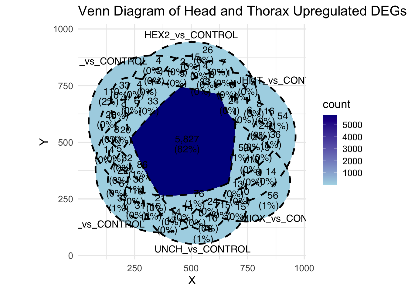
# Display the Venn diagram and datatable for **Head Downregulated DEGs** across contrasts
display_ggvenn_plot(venn_data_down, "Venn Diagram of Head and Thorax Downregulated DEGs - RNAi Contrasts")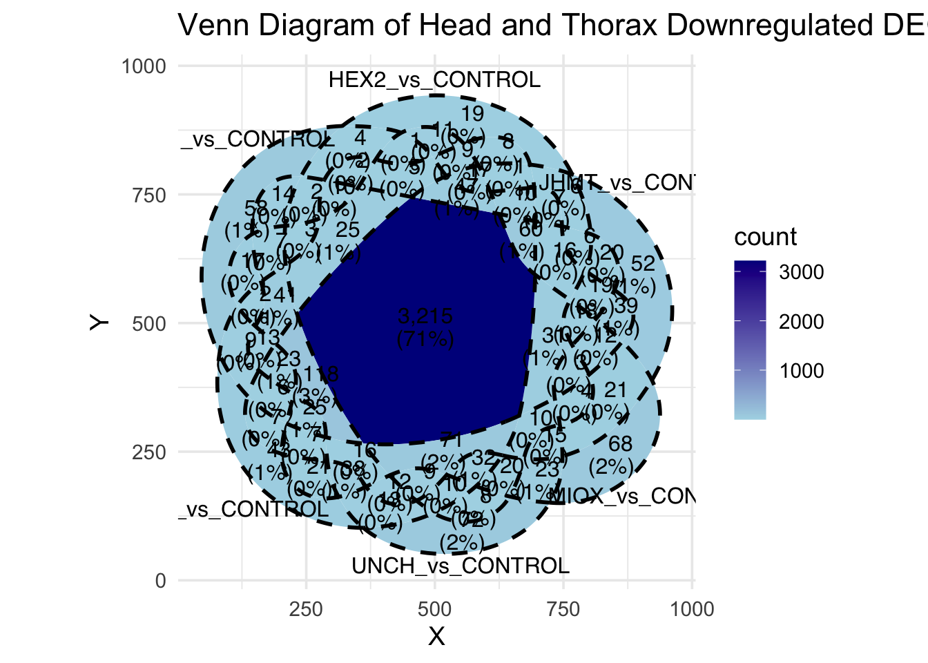
# Display the Venn diagram and datatable for **All Significant DEGs in Head Tissue**
display_ggvenn_plot(venn_data_all, "Venn Diagram of All Significant DEGs in All Tissue - RNAi Contrasts")
# Run the UpSet plot for Head Upregulated DEGs
display_upset_plot(venn_data_up, "UpSet Plot of Head and Thorax Upregulated DEGs - RNAi Contrasts")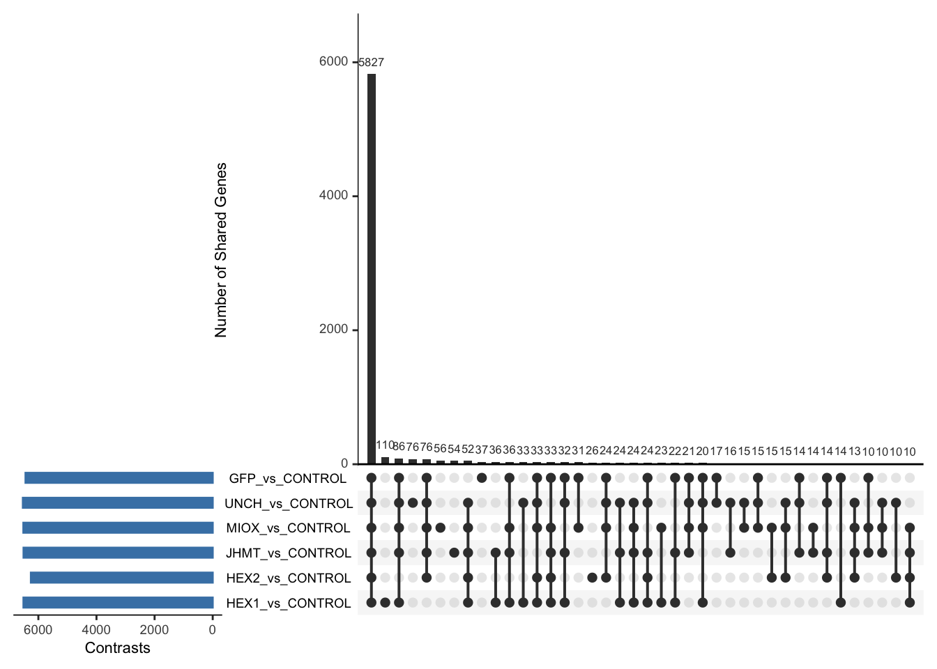
# Run the UpSet plot for Head Downregulated DEGs
display_upset_plot(venn_data_down, "UpSet Plot of Head and Thorax Downregulated DEGs - RNAi Contrasts")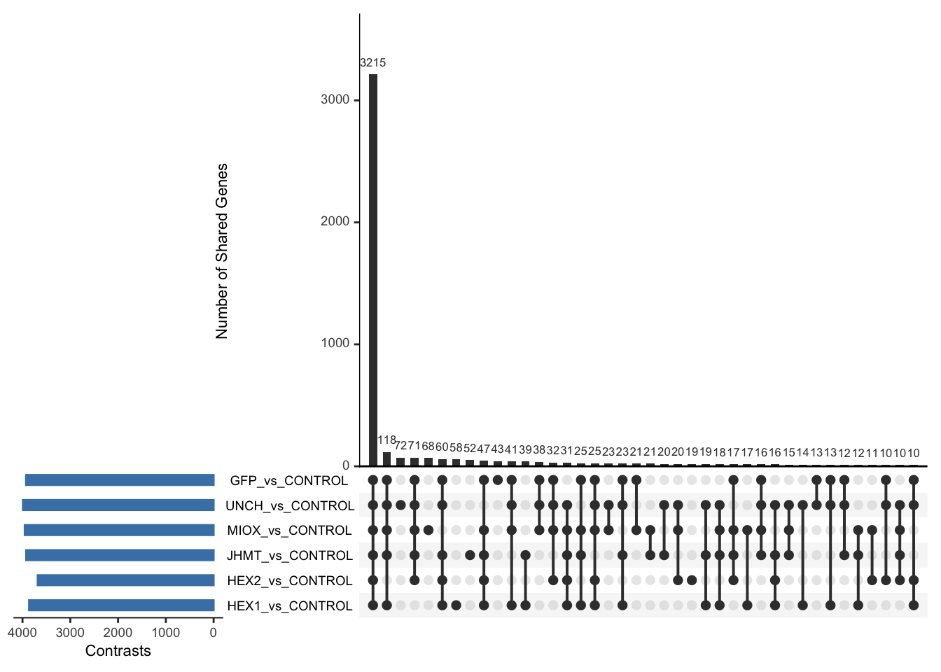
# Run the UpSet plot for Head Upregulated DEGs
display_upset_plot(venn_data_all, "UpSet Plot of All Significant DEGs in All Tissue - RNAi Contrasts")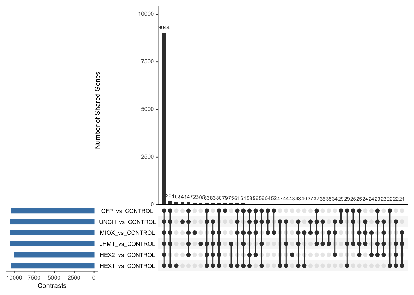
Head tissue
saveDir <- paste0(workDir,"/DEG_results/RNAi/Head_control")
dir.create(saveDir)
### Prepare Sample CSV file #####
samples <- read.delim(file.path(workDir, "list/RNAi/Head_RNAi_noninjectedsample_list.csv"), sep = ",", row.names = 1, header = TRUE)
files <- file.path(workDir, "readcounts/RNAi/", samples$Tissue, samples$Filename)
names(files) <- row.names(samples)
if (all(file.exists(files))) {
message("All the files exist!")
} else {
warning("Some files are missing!")
}All the files exist!### **Standardized Count Matrix Creation**
# Extract all gene lists first
gene_lists <- map(files, function(sample) {
fread(sample, sep = "\t", header = FALSE)[, 1] # Extract Gene IDs (column 1)
})
# Get a unique set of all gene IDs across all samples
all_genes <- unique(unlist(gene_lists))
# Create a named list to store count data with standardized rows
cts_list <- map(files, function(sample) {
data_count <- fread(sample, sep = "\t", header = FALSE)
col_name <- gsub("_counts.txt", "", basename(sample)) # Clean sample name
# Convert to data frame with correct column names
data_count <- setNames(data.frame(data_count[, 1:2]), c("GeneID", col_name))
# Ensure all gene IDs are present (fill missing values with 0)
data_count <- full_join(data.frame(GeneID = all_genes), data_count, by = "GeneID") %>%
mutate(across(where(is.numeric), ~ replace_na(., 0))) # Fill NA with 0
return(data_count)
})
# Merge all samples based on GeneID
cts <- reduce(cts_list, full_join, by = "GeneID")
# Convert to matrix for DESeq2
cts_matrix <- as.matrix(cts[, -1]) # Remove GeneID column for count matrix
rownames(cts_matrix) <- cts$GeneID # Set GeneID as rownames
rm(cts_list) # Free memoryWhile for bulk RNAseq on head and thorax for all species, the DEGs model was made between isolated and crowded individuals (with isolated as the reference state), here, the DEG analysis will be carried between GFP knock-down nymphs (as reference state) vs Hexamerins / Juvenile Hormones / Inositol / Uncharacterized proteins.
### Build DESeq2 Object
dds <- DESeqDataSetFromMatrix(countData = cts_matrix,
colData = samples,
design = ~ Gene)
dds$Gene <- relevel(dds$Gene, ref = "CONTROL")
smallestGroupSize <- 5
keep <- rowSums(counts(dds) >= 10) >= smallestGroupSize
dds <- dds[keep,]
dds <- DESeq(dds)Normalization and PCA
# Plot PCA and investigate quality metrics
vsd <- vst(dds, blind = TRUE)
# Perform PCA
pca_data <- plotPCA(vsd, intgroup = c("Tissue", "Gene"), returnData = TRUE)
# Define colors for genes (slightly transparent) and shapes for tissues
gene_colors <- scale_color_manual(values = alpha(brewer.pal(n = length(unique(pca_data$Gene)), name = "Set1"), 0.8)) # Points are transparent
tissue_shapes <- scale_shape_manual(values = seq(15, 15 + length(unique(pca_data$Tissue))))
# **PCA without labels**
p_pca_nolabel <- ggplot(pca_data, aes(x = PC1, y = PC2, color = Gene, shape = Tissue)) +
geom_point(size = 4) +
gene_colors +
tissue_shapes +
theme_bw() +
theme(legend.title = element_blank(),
legend.text = element_text(face = "bold", size = 14),
axis.text = element_text(size = 12),
axis.title = element_text(size = 14)) +
ggtitle("PCA of All Tissues (No Labels)", subtitle = "Tissues differentiated by shape, Genes by color")
# Save PCA without labels
ggsave(paste0(saveDir, "/PCA_Tissue_Gene_NoLabel.png"), plot = p_pca_nolabel, width = 10, height = 10, dpi = 600, device = "png")
# **PCA with labels**
p_pca_label <- ggplot(pca_data, aes(x = PC1, y = PC2, color = Gene, shape = Tissue)) +
geom_point(size = 4) +
geom_text_repel(aes(label = name), size = 4, color = "black", max.overlaps = 20) + # Labels are fully visible
gene_colors +
tissue_shapes +
theme_bw() +
theme(legend.title = element_blank(),
legend.text = element_text(face = "bold", size = 14),
axis.text = element_text(size = 12),
axis.title = element_text(size = 14)) +
ggtitle("PCA of All Tissues (With Labels)", subtitle = "Tissues differentiated by shape, Genes by color")
# Save PCA with labels
ggsave(paste0(saveDir, "/PCA_Tissue_Gene_Label.png"), plot = p_pca_label, width = 10, height = 10, dpi = 600, device = "png")
# **Return plots for knitr/RMarkdown**
list(NoLabel = p_pca_nolabel, WithLabel = p_pca_label)$NoLabel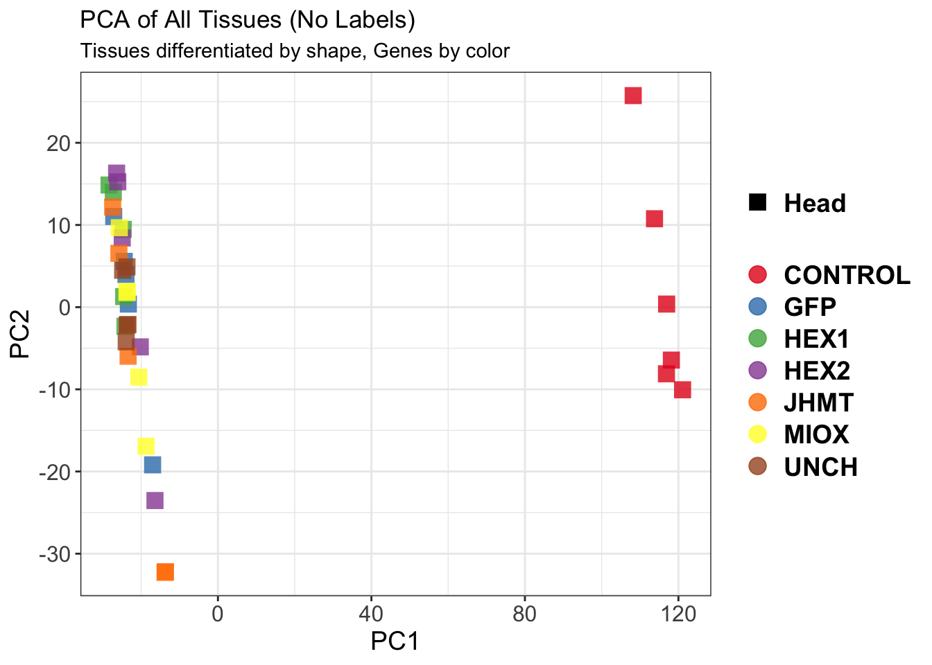
| Version | Author | Date |
|---|---|---|
| b540a1e | Maeva TECHER | 2025-02-27 |
$WithLabel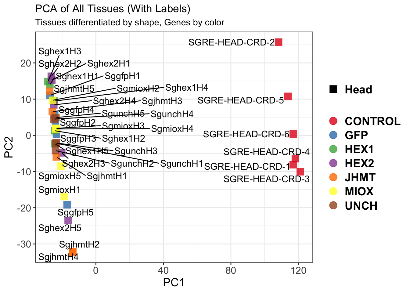
| Version | Author | Date |
|---|---|---|
| b540a1e | Maeva TECHER | 2025-02-27 |
The PCA plot shows clear distinction between tissue types, while gene silencing has a large variation within each tissue, and presents no distinct clear groupings for a single gene.
SVA
### SVA analysis to control for technical variation
dat <- counts(dds, normalized = TRUE)
idx <- rowMeans(dat) > 1
dat <- dat[idx, ]
mod <- model.matrix(~ Gene, colData(dds))
mod0 <- model.matrix(~ 1, colData(dds))
svseq <- svaseq(dat, mod, mod0)Number of significant surrogate variables is: 7
Iteration (out of 5 ):1 2 3 4 5 sva_plots <- create_sva_plots(svseq, dds, saveDir, intgroup = c("Tissue", "Gene"), max_sv = 7)
# Show stripcharts in the report
sva_plots$Stripcharts[[1]] # Show first stripchart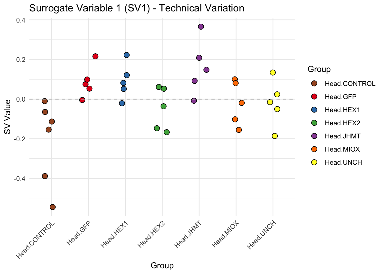
| Version | Author | Date |
|---|---|---|
| b540a1e | Maeva TECHER | 2025-02-27 |
sva_plots$Stripcharts[[2]] # Show second stripchart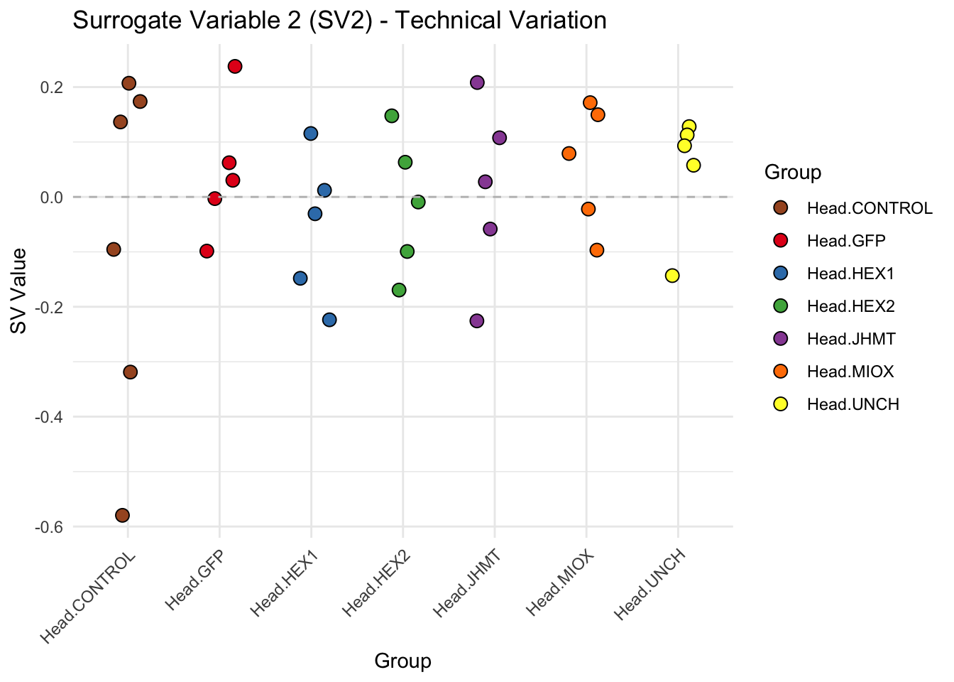
| Version | Author | Date |
|---|---|---|
| b540a1e | Maeva TECHER | 2025-02-27 |
sva_plots$Stripcharts[[3]] # Show third stripchart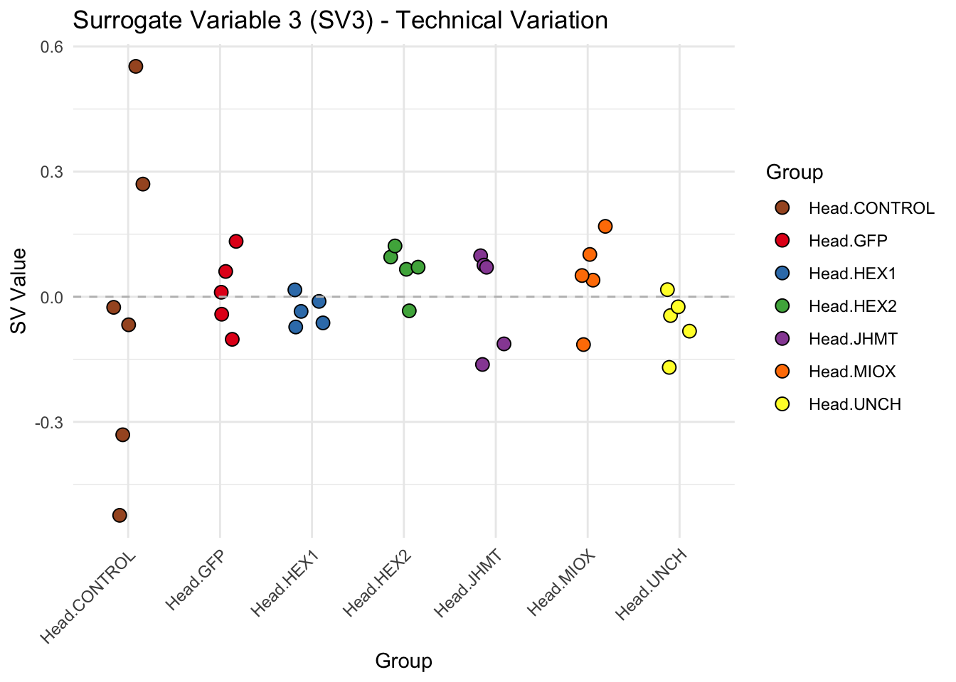
| Version | Author | Date |
|---|---|---|
| b540a1e | Maeva TECHER | 2025-02-27 |
sva_plots$Stripcharts[[4]] 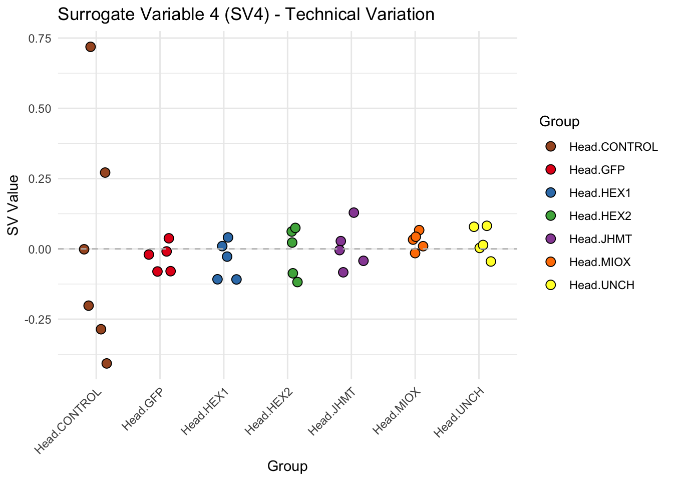
| Version | Author | Date |
|---|---|---|
| b540a1e | Maeva TECHER | 2025-02-27 |
sva_plots$Stripcharts[[5]] # Show second stripchart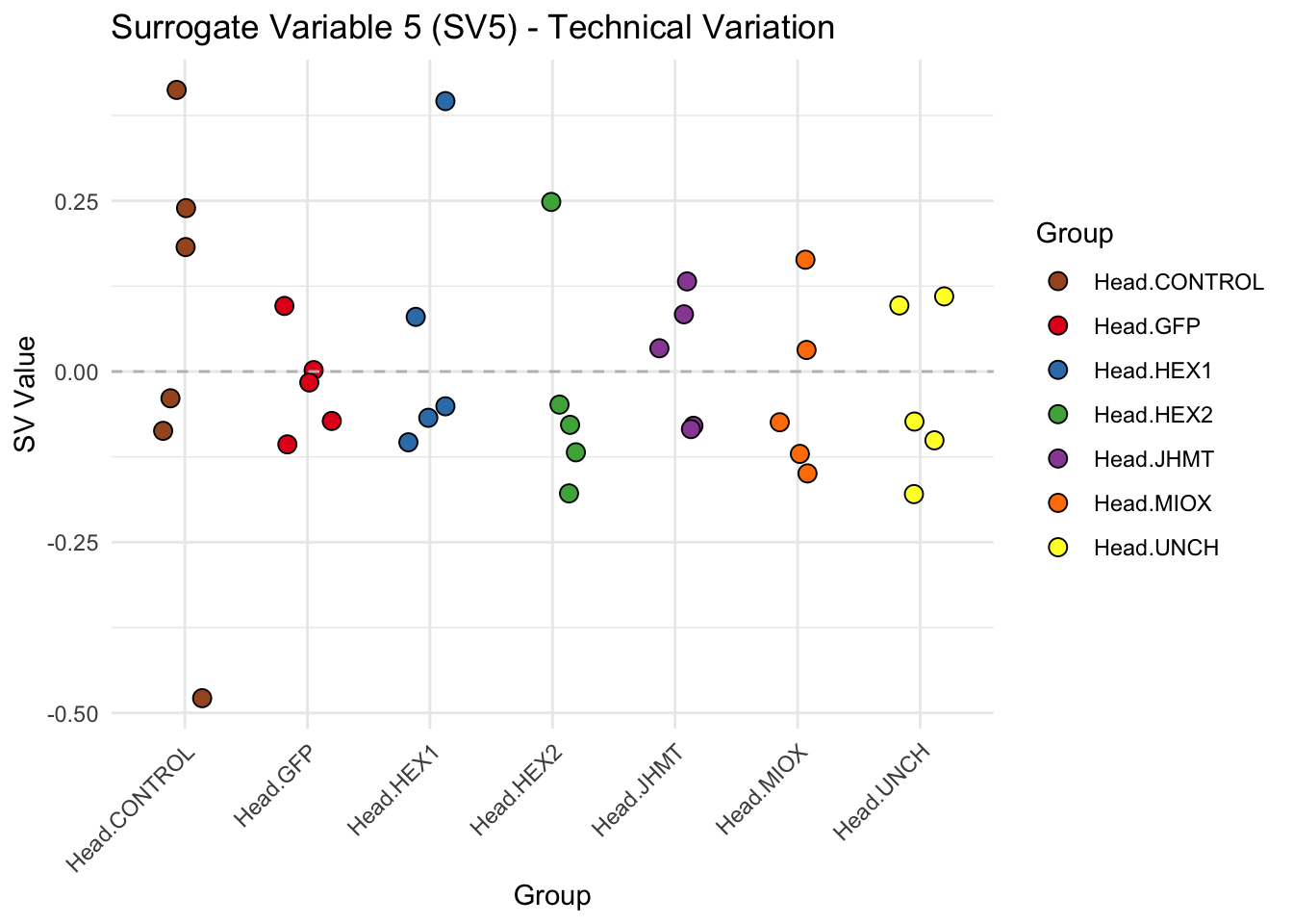
| Version | Author | Date |
|---|---|---|
| b540a1e | Maeva TECHER | 2025-02-27 |
sva_plots$Stripcharts[[6]] # Show third stripchart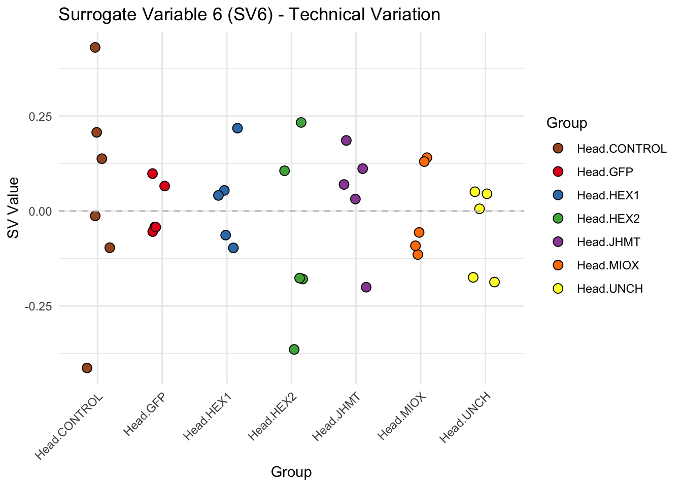
| Version | Author | Date |
|---|---|---|
| b540a1e | Maeva TECHER | 2025-02-27 |
sva_plots$Stripcharts[[7]] 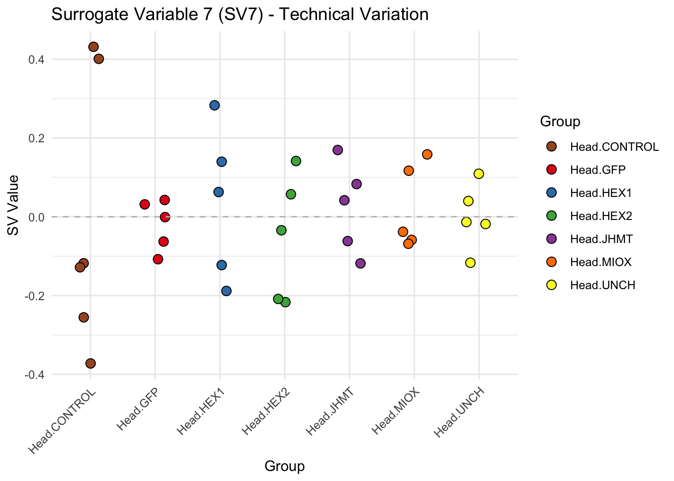
| Version | Author | Date |
|---|---|---|
| b540a1e | Maeva TECHER | 2025-02-27 |
# Show scatter plots in the report
sva_plots$ScatterPlots[["1_2"]] # Show SV1 vs SV2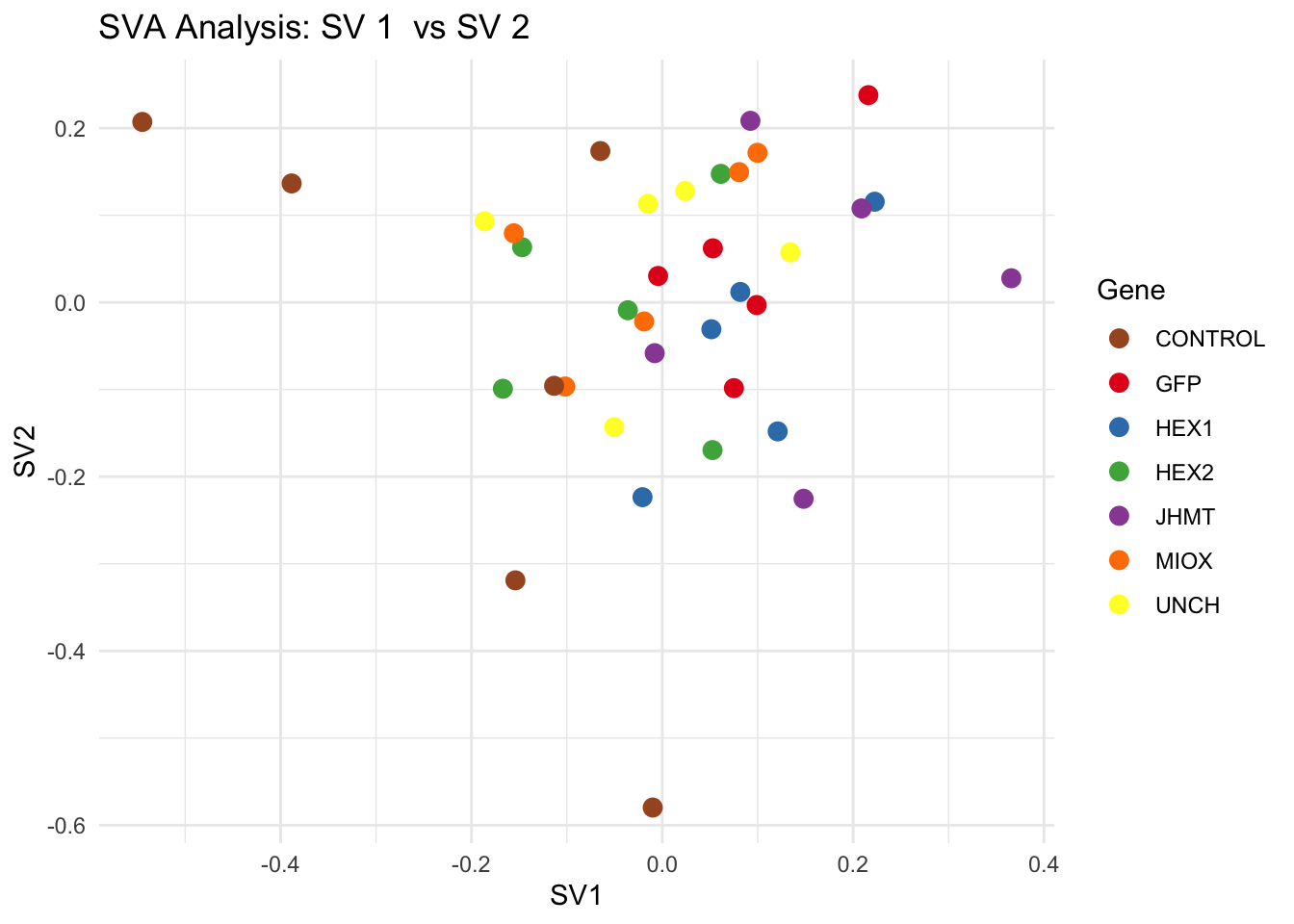
| Version | Author | Date |
|---|---|---|
| b540a1e | Maeva TECHER | 2025-02-27 |
sva_plots$ScatterPlots[["1_3"]] # Show SV1 vs SV3
| Version | Author | Date |
|---|---|---|
| b540a1e | Maeva TECHER | 2025-02-27 |
sva_plots$ScatterPlots[["2_3"]] # Show SV2 vs SV3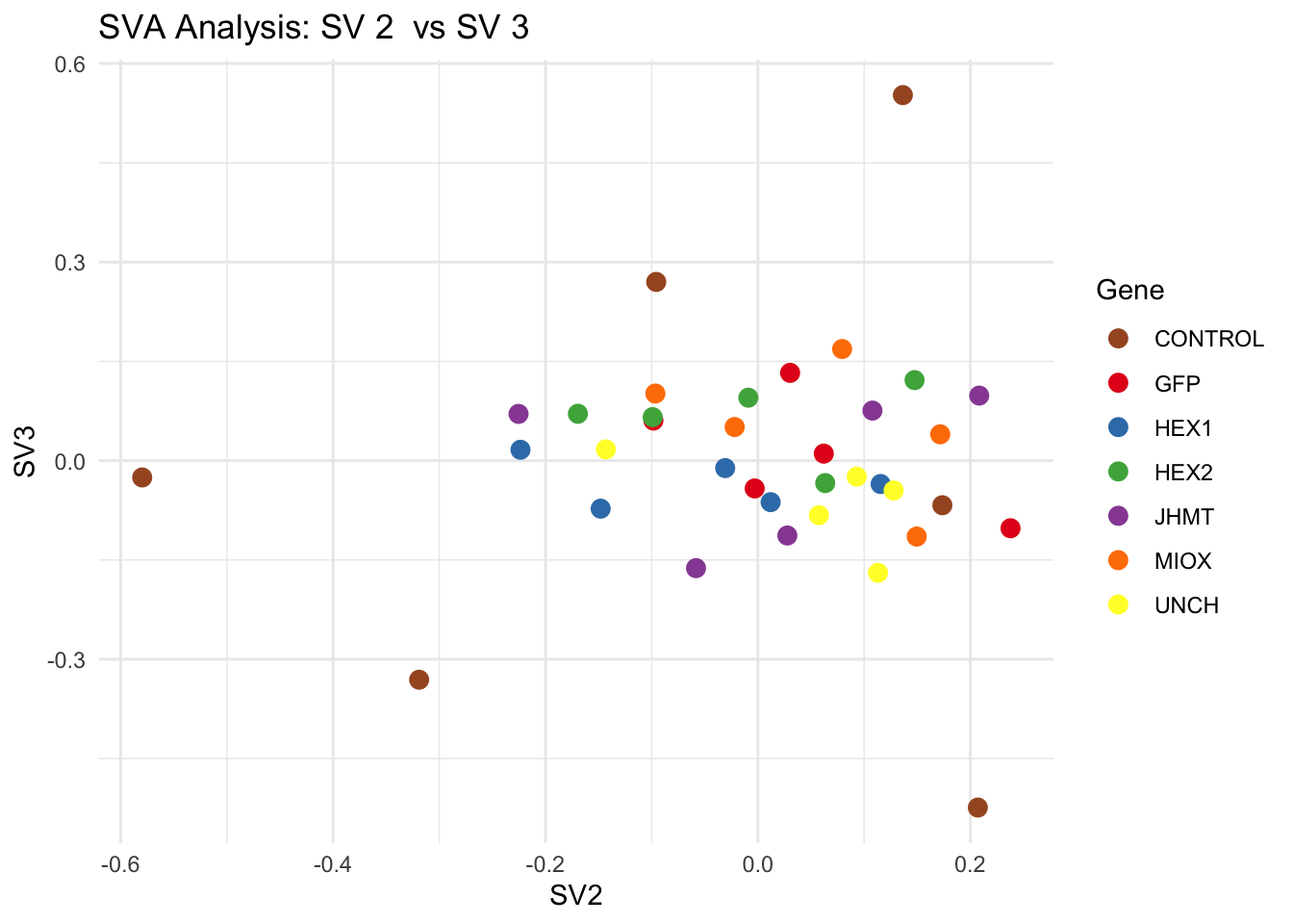
SV1 is clearly showing an effect of tissue. We rerun the
DESeq2 model but this time including the surrogate variable
SV2 and SV3 as a covariates only, as we know that the modeled variation
is more likely explained by tissue and gene variation rather than batch
effects.
ddssva <- dds
ddssva$SV1 <- svseq$sv[,1]
ddssva$SV2 <- svseq$sv[,2]
ddssva$SV3 <- svseq$sv[,3]
ddssva$SV4 <- svseq$sv[,4]
ddssva$SV5 <- svseq$sv[,5]
ddssva$SV6 <- svseq$sv[,6]
ddssva$SV7 <- svseq$sv[,7]
design(ddssva) <- ~ SV1 + SV2 + SV3 + SV4 + SV5 + SV6 + SV7 + Gene
ddssva$Gene <- relevel(ddssva$Gene, ref = "CONTROL")
smallestGroupSize <- 5
keep <- rowSums(counts(ddssva) >= 10) >= smallestGroupSize
ddssva <- ddssva[keep,]
ddssva <- DESeq(ddssva)
ddssva <- ddssva[which(mcols(ddssva)$betaConv),] # remove non converging rows
### Extract results
message("Available contrasts are: ", paste(resultsNames(ddssva), collapse = ", "))
hex1 <- results(ddssva, contrast = c("Gene", "HEX1", "CONTROL"), alpha = 0.05)
hex2 <- results(ddssva, contrast = c("Gene", "HEX2", "CONTROL"), alpha = 0.05)
jhmt <- results(ddssva, contrast = c("Gene", "JHMT", "CONTROL"), alpha = 0.05)
miox <- results(ddssva, contrast = c("Gene", "MIOX", "CONTROL"), alpha = 0.05)
unch <- results(ddssva, contrast = c("Gene", "UNCH", "CONTROL"), alpha = 0.05)
gfp <- results(ddssva, contrast = c("Gene", "GFP", "CONTROL"), alpha = 0.05)Volcano plots and Heatmaps
# Define contrast_sets
hex1_samples <- c("SGRE-HEAD-CRD-1","SGRE-HEAD-CRD-2","SGRE-HEAD-CRD-3","SGRE-HEAD-CRD-4","SGRE-HEAD-CRD-5",
"SGRE-HEAD-CRD-6","SggfpH1","SggfpH2","SggfpH3","SggfpH4","SggfpH5",
"Sghex1H1","Sghex1H2","Sghex1H3","Sghex1H4","Sghex1H5")
hex2_samples <- c("SGRE-HEAD-CRD-1","SGRE-HEAD-CRD-2","SGRE-HEAD-CRD-3","SGRE-HEAD-CRD-4","SGRE-HEAD-CRD-5",
"SGRE-HEAD-CRD-6","SggfpH1","SggfpH2","SggfpH3","SggfpH4","SggfpH5",
"Sghex2H1","Sghex2H2","Sghex2H3","Sghex2H4","Sghex2H5")
jhmt_samples <- c("SGRE-HEAD-CRD-1","SGRE-HEAD-CRD-2","SGRE-HEAD-CRD-3","SGRE-HEAD-CRD-4","SGRE-HEAD-CRD-5",
"SGRE-HEAD-CRD-6","SggfpH1","SggfpH2","SggfpH3","SggfpH4","SggfpH5",
"SgjhmtH1","SgjhmtH2","SgjhmtH3","SgjhmtH4","SgjhmtH5")
miox_samples <- c("SGRE-HEAD-CRD-1","SGRE-HEAD-CRD-2","SGRE-HEAD-CRD-3","SGRE-HEAD-CRD-4","SGRE-HEAD-CRD-5",
"SGRE-HEAD-CRD-6","SggfpH1","SggfpH2","SggfpH3","SggfpH4","SggfpH5",
"SgmioxH1","SgmioxH2","SgmioxH3","SgmioxH4","SgmioxH5")
unch_samples <- c("SGRE-HEAD-CRD-1","SGRE-HEAD-CRD-2","SGRE-HEAD-CRD-3","SGRE-HEAD-CRD-4","SGRE-HEAD-CRD-5",
"SGRE-HEAD-CRD-6","SggfpH1","SggfpH2","SggfpH3","SggfpH4","SggfpH5",
"SgunchH1","SgunchH2","SgunchH3","SgunchH4","SgunchH5")
gfp_samples <- c("SGRE-HEAD-CRD-1","SGRE-HEAD-CRD-2","SGRE-HEAD-CRD-3","SGRE-HEAD-CRD-4","SGRE-HEAD-CRD-5",
"SGRE-HEAD-CRD-6","SggfpH1","SggfpH2","SggfpH3","SggfpH4","SggfpH5")
# Run full analysis
hex1_plots <- visualize_data_nopng(hex1, "HEX1_vs_CONTROL", hex1_samples)
hex2_plots <- visualize_data_nopng(hex2, "HEX2_vs_CONTROL", hex2_samples)
jhmt_plots <- visualize_data_nopng(jhmt, "JHMT_vs_CONTROL", jhmt_samples)
miox_plots <- visualize_data_nopng(miox, "MIOX_vs_CONTROL", miox_samples)
unch_plots <- visualize_data_nopng(unch, "UNCH_vs_CONTROL", unch_samples)
gfp_plots <- visualize_data_nopng(gfp, "GFP_vs_CONTROL", gfp_samples)
hex1_plots$volcano; hex1_plots$heatmap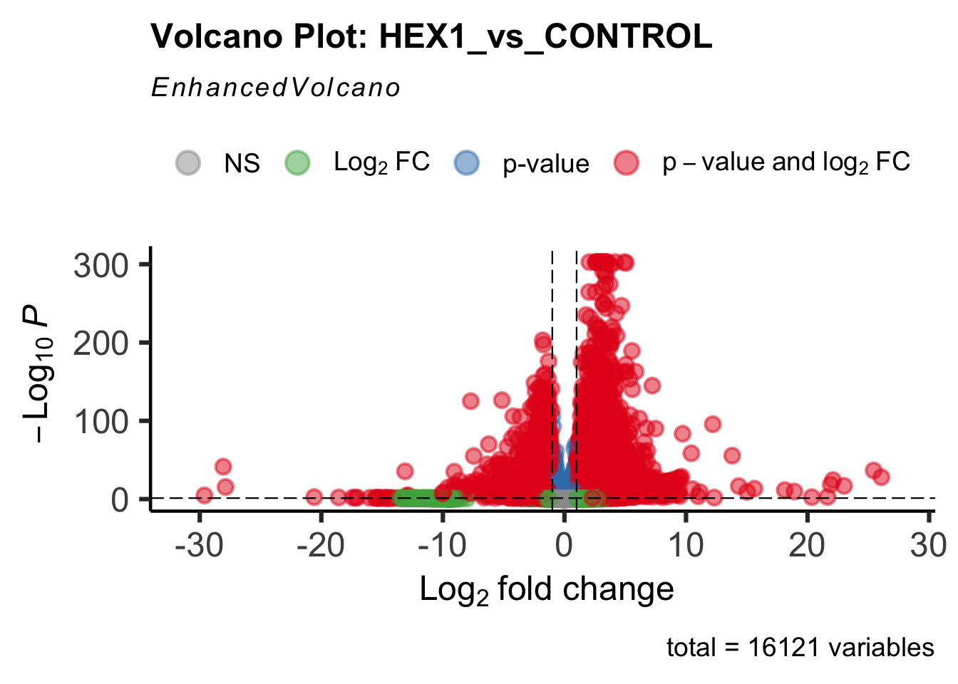
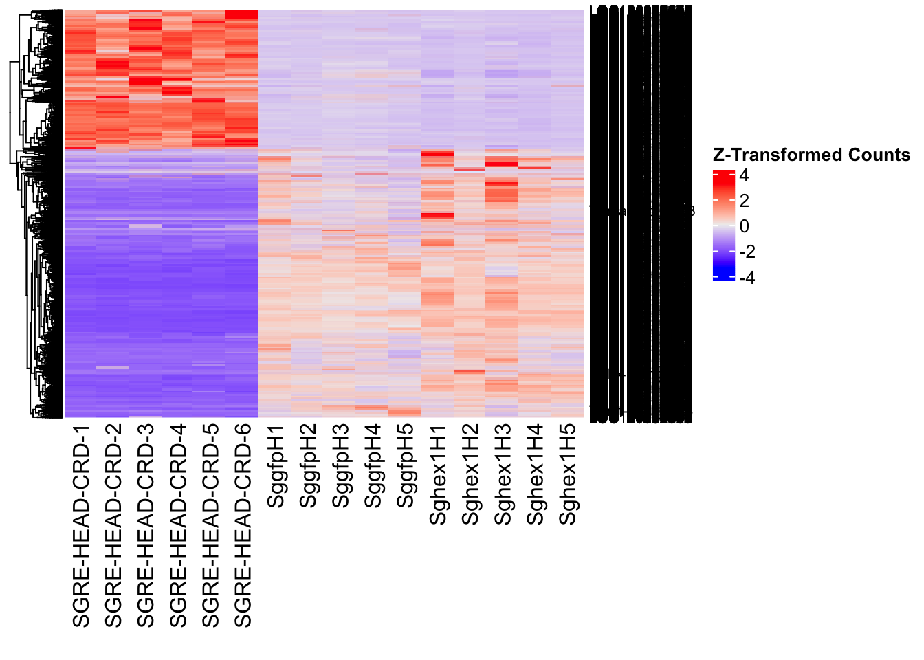
| Version | Author | Date |
|---|---|---|
| b540a1e | Maeva TECHER | 2025-02-27 |
hex2_plots$volcano; hex2_plots$heatmap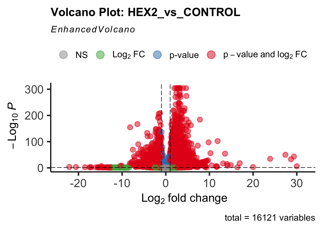

| Version | Author | Date |
|---|---|---|
| b540a1e | Maeva TECHER | 2025-02-27 |
jhmt_plots$volcano; jhmt_plots$heatmap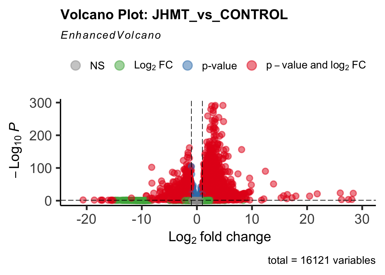
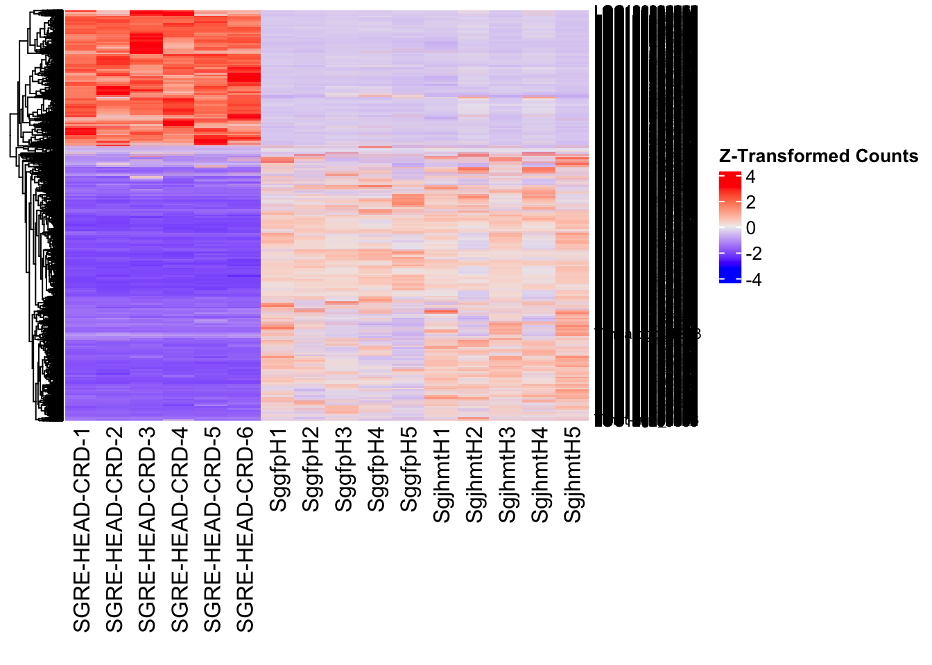
| Version | Author | Date |
|---|---|---|
| b540a1e | Maeva TECHER | 2025-02-27 |
miox_plots$volcano; miox_plots$heatmap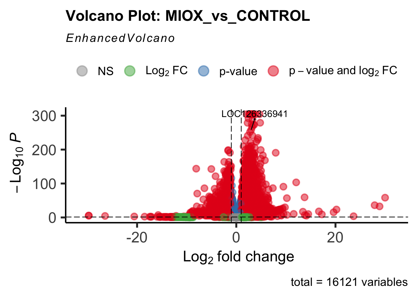
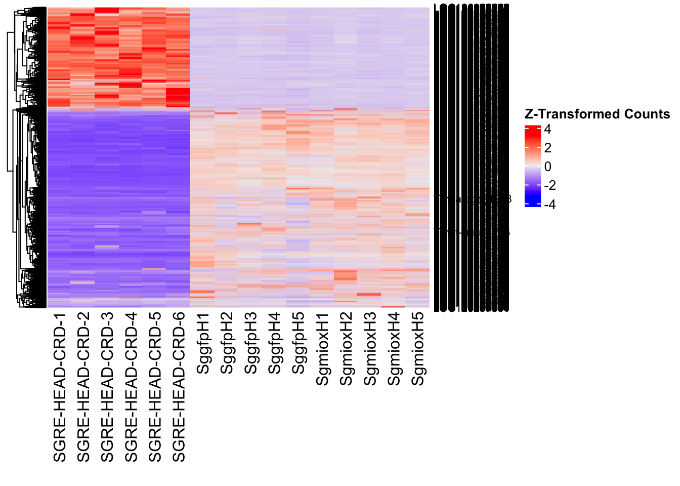
| Version | Author | Date |
|---|---|---|
| b540a1e | Maeva TECHER | 2025-02-27 |
unch_plots$volcano; unch_plots$heatmap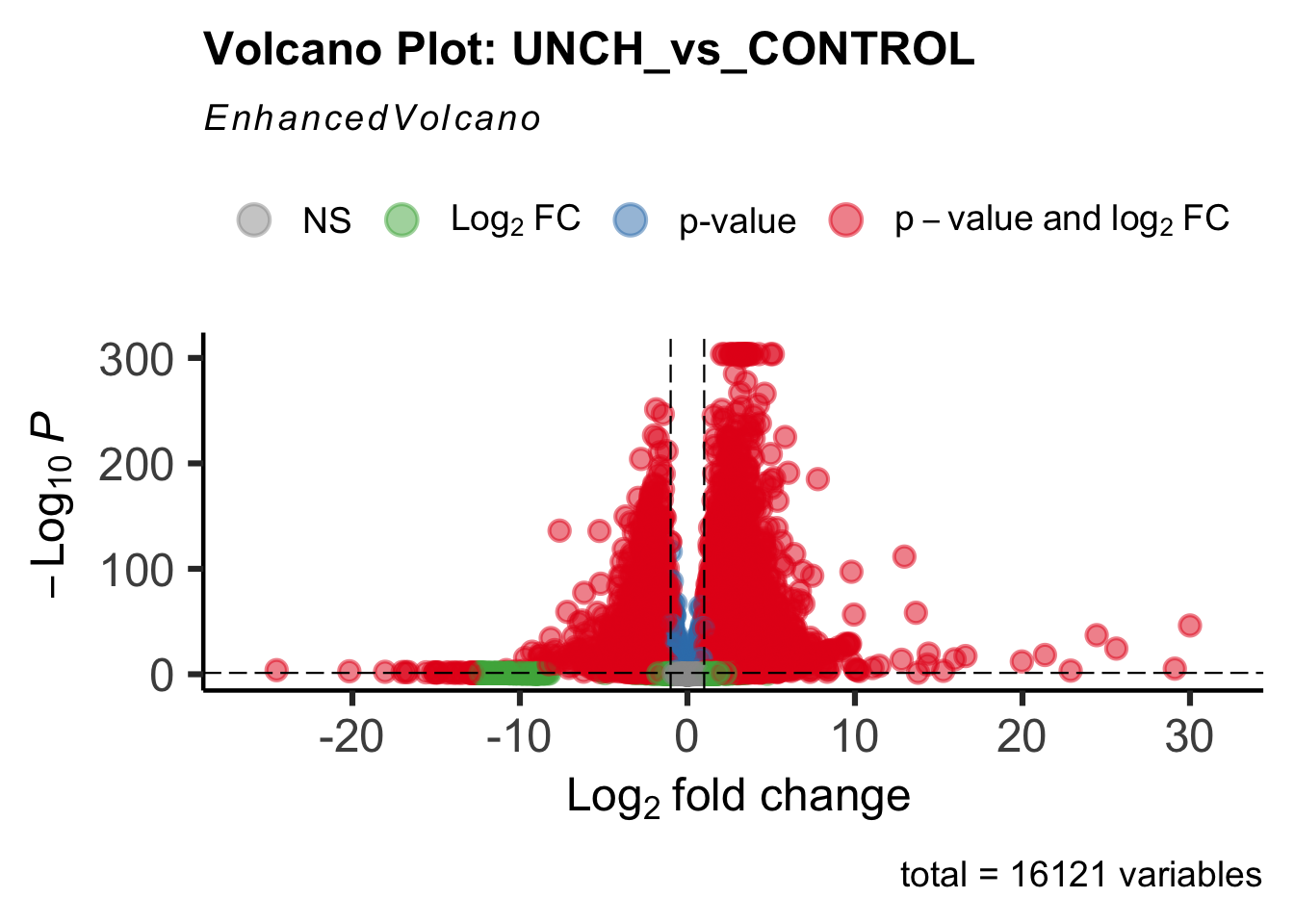
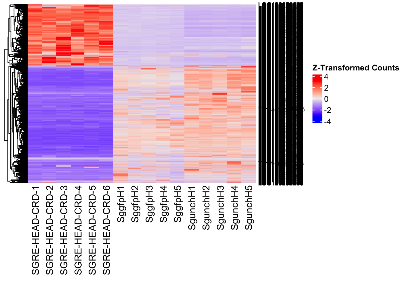
| Version | Author | Date |
|---|---|---|
| b540a1e | Maeva TECHER | 2025-02-27 |
gfp_plots$volcano; gfp_plots$heatmap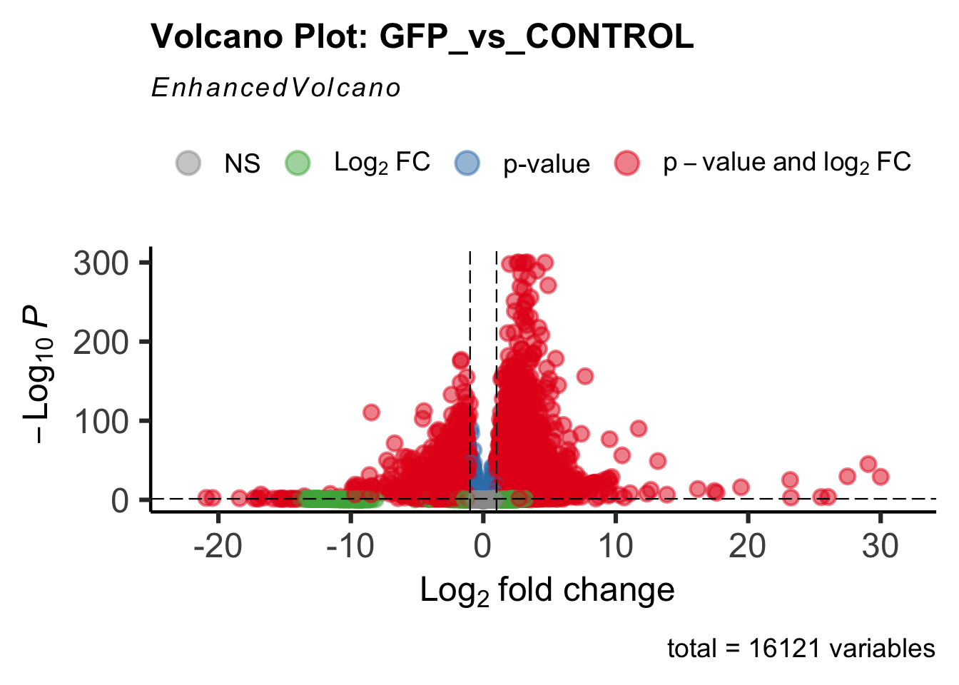
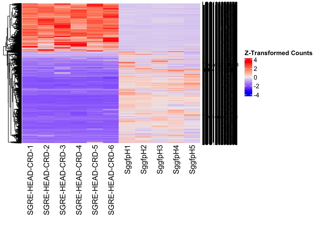
DEG tables
The following tables show the genes differentially expressed with at least an absolute log2fold change of > 1 considering Head tissues only. Considering GFP as the reference state, upregulated genes in knockdown treatment in red and downregulated genes in knockdown treatment in blue. You can search for a gene of interest by writting a LOCID or description in the search bar or sort by column.
# Generate tables for each contrast
table_hex1 <- generate_deg_table(ddssva, "Gene_HEX1_vs_CONTROL", allspecies_df)
out of 16121 with nonzero total read count
adjusted p-value < 0.05
LFC > 0 (up) : 7836, 49%
LFC < 0 (down) : 4830, 30%
outliers [1] : 0, 0%
low counts [2] : 0, 0%
(mean count < 2)
[1] see 'cooksCutoff' argument of ?results
[2] see 'independentFiltering' argument of ?resultsTotal DEGs p-value < 0.05 and absolute logFoldChange > 1: 9521LFC > 1 (up) : 6258 (65.73%)LFC < -1 (down) : 3263 (34.27%)table_hex1$kable_tabletable_hex2 <- generate_deg_table(ddssva, "Gene_HEX2_vs_CONTROL", allspecies_df)
out of 16121 with nonzero total read count
adjusted p-value < 0.05
LFC > 0 (up) : 7655, 47%
LFC < 0 (down) : 4879, 30%
outliers [1] : 0, 0%
low counts [2] : 0, 0%
(mean count < 2)
[1] see 'cooksCutoff' argument of ?results
[2] see 'independentFiltering' argument of ?resultsTotal DEGs p-value < 0.05 and absolute logFoldChange > 1: 8961LFC > 1 (up) : 5969 (66.61%)LFC < -1 (down) : 2992 (33.39%)table_hex2$kable_tabletable_jhmt <- generate_deg_table(ddssva, "Gene_JHMT_vs_CONTROL", allspecies_df)
out of 16121 with nonzero total read count
adjusted p-value < 0.05
LFC > 0 (up) : 7510, 47%
LFC < 0 (down) : 4678, 29%
outliers [1] : 0, 0%
low counts [2] : 0, 0%
(mean count < 2)
[1] see 'cooksCutoff' argument of ?results
[2] see 'independentFiltering' argument of ?resultsTotal DEGs p-value < 0.05 and absolute logFoldChange > 1: 9012LFC > 1 (up) : 6015 (66.74%)LFC < -1 (down) : 2997 (33.26%)table_jhmt$kable_tabletable_miox <- generate_deg_table(ddssva, "Gene_MIOX_vs_CONTROL", allspecies_df)
out of 16121 with nonzero total read count
adjusted p-value < 0.05
LFC > 0 (up) : 7810, 48%
LFC < 0 (down) : 4879, 30%
outliers [1] : 0, 0%
low counts [2] : 0, 0%
(mean count < 2)
[1] see 'cooksCutoff' argument of ?results
[2] see 'independentFiltering' argument of ?resultsTotal DEGs p-value < 0.05 and absolute logFoldChange > 1: 9316LFC > 1 (up) : 6163 (66.16%)LFC < -1 (down) : 3153 (33.84%)table_miox$kable_tabletable_unch <- generate_deg_table(ddssva, "Gene_UNCH_vs_CONTROL", allspecies_df)
out of 16121 with nonzero total read count
adjusted p-value < 0.05
LFC > 0 (up) : 8065, 50%
LFC < 0 (down) : 4966, 31%
outliers [1] : 0, 0%
low counts [2] : 0, 0%
(mean count < 2)
[1] see 'cooksCutoff' argument of ?results
[2] see 'independentFiltering' argument of ?resultsTotal DEGs p-value < 0.05 and absolute logFoldChange > 1: 9870LFC > 1 (up) : 6462 (65.47%)LFC < -1 (down) : 3408 (34.53%)table_unch$kable_tabletable_gfp <- generate_deg_table(ddssva, "Gene_GFP_vs_CONTROL", allspecies_df)
out of 16121 with nonzero total read count
adjusted p-value < 0.05
LFC > 0 (up) : 7538, 47%
LFC < 0 (down) : 4762, 30%
outliers [1] : 0, 0%
low counts [2] : 0, 0%
(mean count < 2)
[1] see 'cooksCutoff' argument of ?results
[2] see 'independentFiltering' argument of ?resultsTotal DEGs p-value < 0.05 and absolute logFoldChange > 1: 9067LFC > 1 (up) : 5974 (65.89%)LFC < -1 (down) : 3093 (34.11%)table_gfp$kable_tableSummary and Overlap
# Summarize DEGs for all contrasts
deg_summary <- bind_rows(
summarize_deg_counts(table_hex1, "HEX1 vs CONTROL"),
summarize_deg_counts(table_hex2, "HEX2 vs CONTROL"),
summarize_deg_counts(table_jhmt, "JHMT vs CONTROL"),
summarize_deg_counts(table_miox, "MIOX vs CONTROL"),
summarize_deg_counts(table_unch, "UNCH vs CONTROL"),
summarize_deg_counts(table_gfp, "GFP vs CONTROL")
)
# Display table using kable with styling
deg_summary %>%
kable("html", escape = FALSE, col.names = gsub("_", " ", names(.))) %>%
kable_styling("striped", full_width = TRUE) %>%
column_spec(2, color = "red", bold = TRUE) %>% # Upregulated in red
column_spec(3, color = "blue", bold = TRUE) %>% # Downregulated in blue
add_header_above(c("Summary of DEGs" = 3)) %>%
row_spec(0, bold = TRUE)| Contrast | Upregulated | Downregulated |
|---|---|---|
| HEX1 vs CONTROL | 6209 | 3241 |
| HEX2 vs CONTROL | 5921 | 2961 |
| JHMT vs CONTROL | 5965 | 2969 |
| MIOX vs CONTROL | 6118 | 3123 |
| UNCH vs CONTROL | 6427 | 3384 |
| GFP vs CONTROL | 5921 | 3074 |
# Define the list of RNAi contrasts
contrast_list <- c("HEX1_vs_CONTROL", "HEX2_vs_CONTROL", "JHMT_vs_CONTROL",
"MIOX_vs_CONTROL", "UNCH_vs_CONTROL", "GFP_vs_CONTROL")
# Initialize empty lists for storing Head-specific DEGs for each contrast
venn_data_up <- list()
venn_data_down <- list()
venn_data_all <- list()
# Function to load Head-specific DEGs for a given set of contrasts
load_deg_contrasts_head <- function(contrast_list) {
degs_up <- list()
degs_down <- list()
degs_all <- list()
for (contrast in contrast_list) {
deg_file <- file.path(workDir, "DEG_results/RNAi/Head_control/", contrast, paste0("DEG_sigresults_", contrast, ".csv"))
if (!file.exists(deg_file)) {
message(paste("File missing for contrast:", contrast))
next # Skip if the file doesn't exist
}
deg_data <- read.csv(deg_file, stringsAsFactors = FALSE)
# Convert row names to a column if necessary
if ("X" %in% colnames(deg_data)) {
colnames(deg_data)[colnames(deg_data) == "X"] <- "GeneID"
}
# Check if data is empty
if (nrow(deg_data) == 0) {
message(paste("No data for contrast:", contrast))
next
}
# Select significant DEGs (Up, Down, All)
degs_up[[contrast]] <- deg_data %>%
filter(padj < 0.05 & log2FoldChange >= 1) %>%
pull(GeneID) # Extract GeneID column
degs_down[[contrast]] <- deg_data %>%
filter(padj < 0.05 & log2FoldChange <= -1) %>%
pull(GeneID) # Extract GeneID column
degs_all[[contrast]] <- deg_data %>%
filter(padj < 0.05 & abs(log2FoldChange) >= 1) %>%
pull(GeneID) # Extract GeneID column
}
return(list(up = degs_up, down = degs_down, all = degs_all))
}
# Load DEG data for the defined contrasts (Head tissue only)
venn_data_contrasts <- load_deg_contrasts_head(contrast_list)
# Prepare the data for the Venn diagrams
venn_data_up <- venn_data_contrasts$up
venn_data_down <- venn_data_contrasts$down
venn_data_all <- venn_data_contrasts$all
# Display the Venn diagram and datatable for **Head Upregulated DEGs** across contrasts
display_ggvenn_plot(venn_data_up, "Venn Diagram of Head Upregulated DEGs - RNAi Contrasts")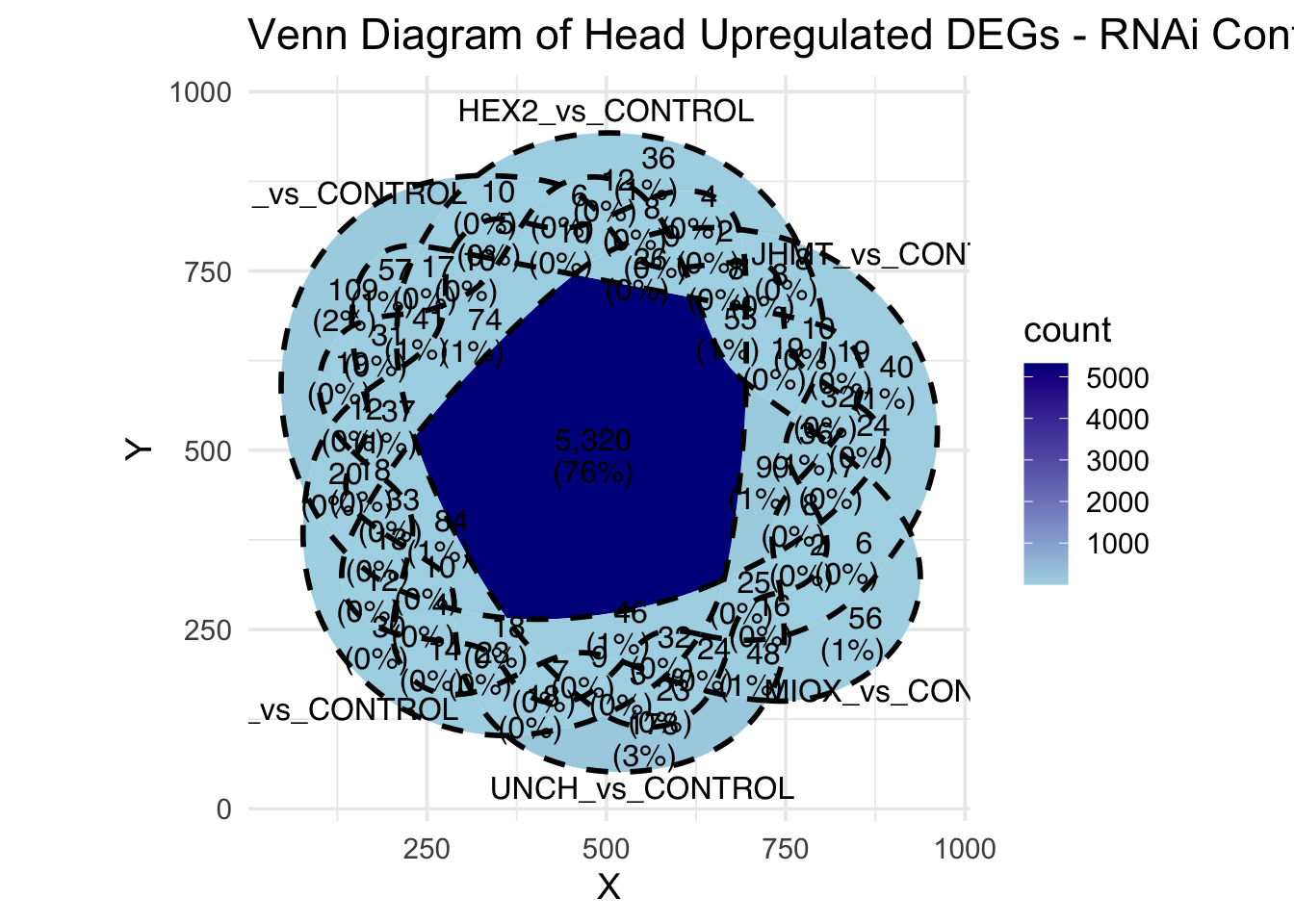
# Display the Venn diagram and datatable for **Head Downregulated DEGs** across contrasts
display_ggvenn_plot(venn_data_down, "Venn Diagram of Head Downregulated DEGs - RNAi Contrasts")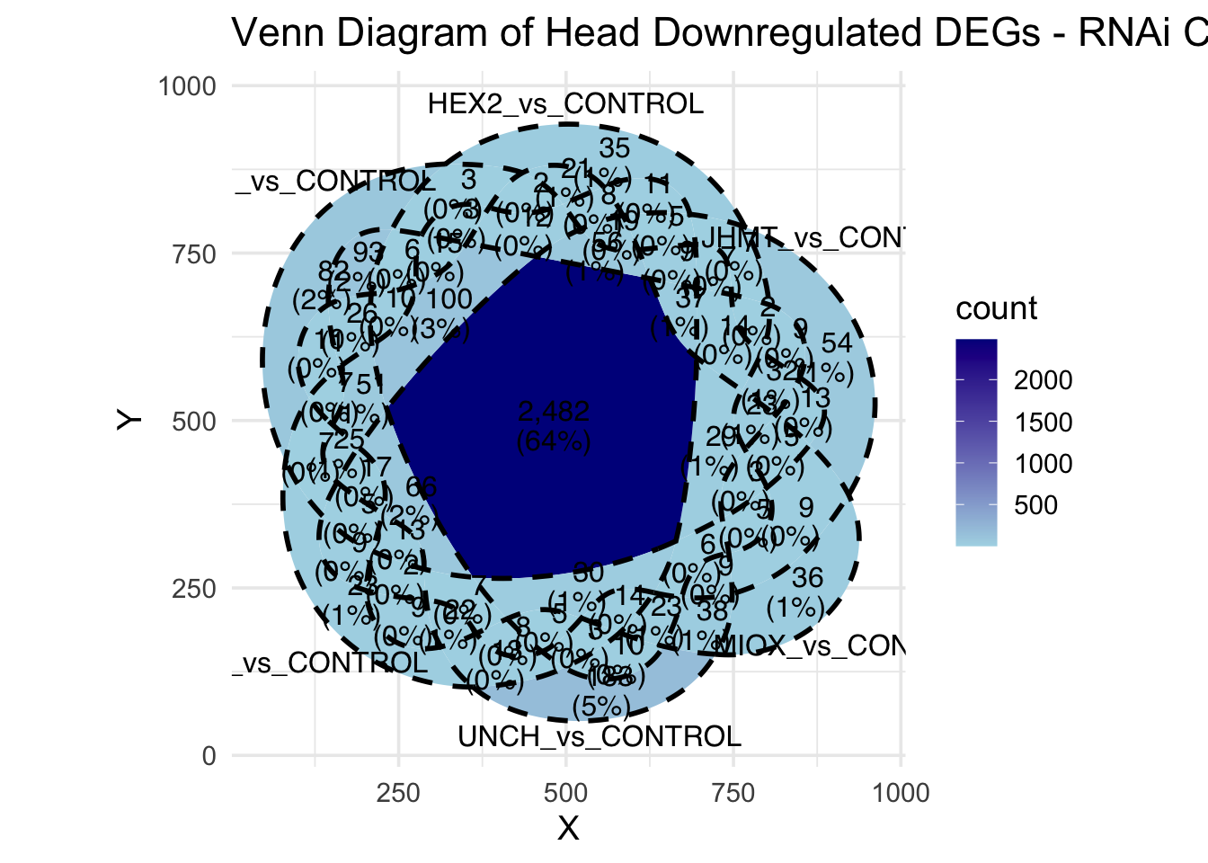
# Display the Venn diagram and datatable for **All Significant DEGs in Head Tissue**
display_ggvenn_plot(venn_data_all, "Venn Diagram of All Significant DEGs in Head Tissue - RNAi Contrasts")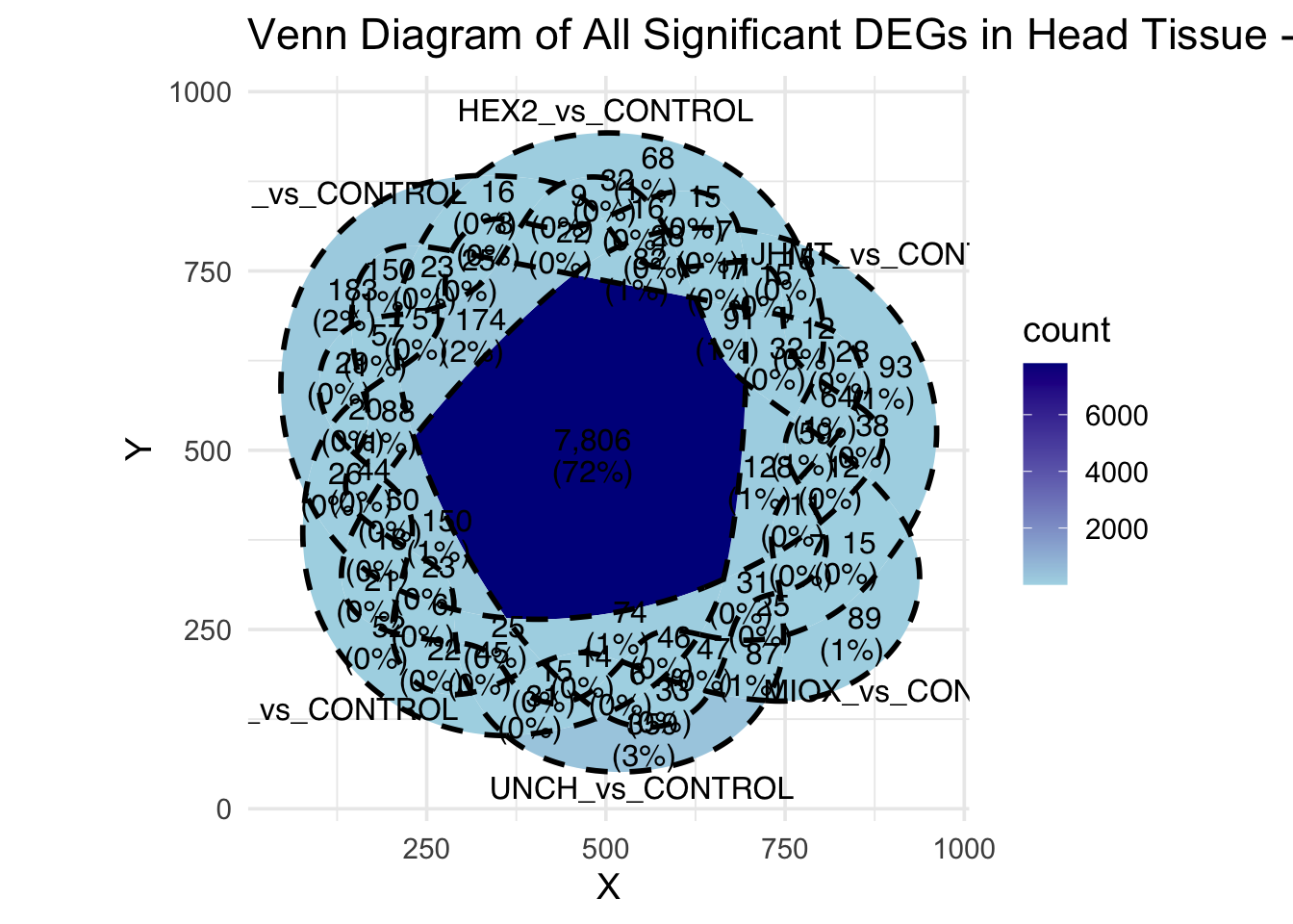
# Run the UpSet plot for Head Upregulated DEGs
display_upset_plot(venn_data_up, "UpSet Plot of Head Upregulated DEGs - RNAi Contrasts")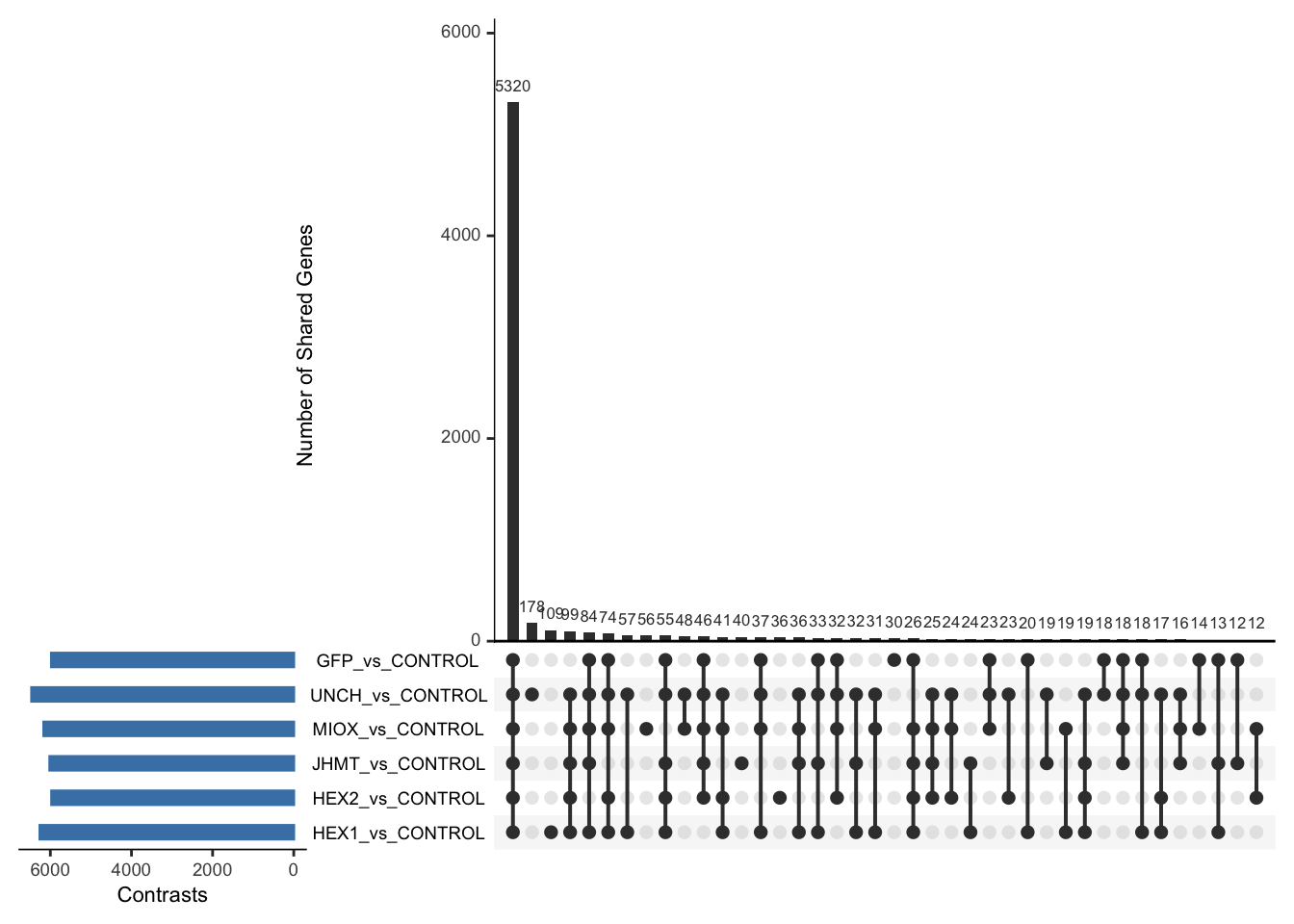
# Run the UpSet plot for Head Downregulated DEGs
display_upset_plot(venn_data_down, "UpSet Plot of Head Downregulated DEGs - RNAi Contrasts")
# Run the UpSet plot for Head Upregulated DEGs
display_upset_plot(venn_data_down, "UpSet Plot of All Significant DEGs in Head Tissue - RNAi Contrasts")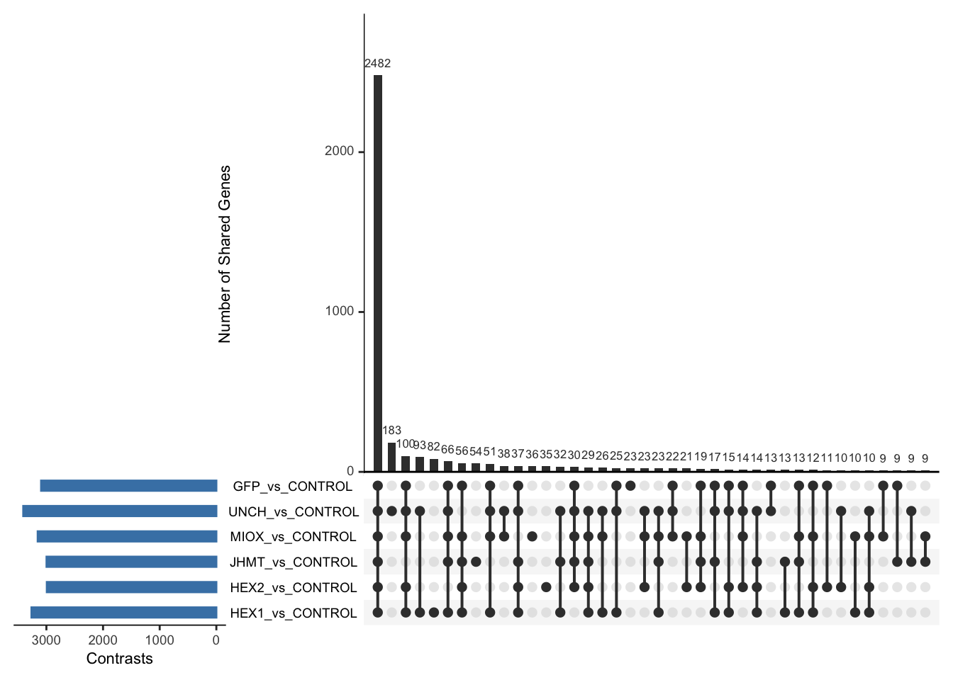
Thorax tissue
saveDir <- paste0(workDir,"/DEG_results/RNAi/Thorax_control")
dir.create(saveDir)
### Prepare Sample CSV file #####
samples <- read.delim(file.path(workDir, "list/RNAi/Thorax_RNAi_noninjectedsample_list.csv"), sep = ",", row.names = 1, header = TRUE)
files <- file.path(workDir, "readcounts/RNAi/", samples$Tissue, samples$Filename)
names(files) <- row.names(samples)
if (all(file.exists(files))) {
message("All the files exist!")
} else {
warning("Some files are missing!")
}All the files exist!### **Standardized Count Matrix Creation**
# Extract all gene lists first
gene_lists <- map(files, function(sample) {
fread(sample, sep = "\t", header = FALSE)[, 1] # Extract Gene IDs (column 1)
})
# Get a unique set of all gene IDs across all samples
all_genes <- unique(unlist(gene_lists))
# Create a named list to store count data with standardized rows
cts_list <- map(files, function(sample) {
data_count <- fread(sample, sep = "\t", header = FALSE)
col_name <- gsub("_counts.txt", "", basename(sample)) # Clean sample name
# Convert to data frame with correct column names
data_count <- setNames(data.frame(data_count[, 1:2]), c("GeneID", col_name))
# Ensure all gene IDs are present (fill missing values with 0)
data_count <- full_join(data.frame(GeneID = all_genes), data_count, by = "GeneID") %>%
mutate(across(where(is.numeric), ~ replace_na(., 0))) # Fill NA with 0
return(data_count)
})
# Merge all samples based on GeneID
cts <- reduce(cts_list, full_join, by = "GeneID")
# Convert to matrix for DESeq2
cts_matrix <- as.matrix(cts[, -1]) # Remove GeneID column for count matrix
rownames(cts_matrix) <- cts$GeneID # Set GeneID as rownames
rm(cts_list) # Free memoryWhile for bulk RNAseq on head and thorax for all species, the DEGs model was made between isolated and crowded individuals (with isolated as the reference state), here, the DEG analysis will be carried between GFP knock-down nymphs (as reference state) vs Hexamerins / Juvenile Hormones / Inositol / Uncharacterized proteins.
### Build DESeq2 Object
dds <- DESeqDataSetFromMatrix(countData = cts_matrix,
colData = samples,
design = ~ Gene)
dds$Gene <- relevel(dds$Gene, ref = "CONTROL")
smallestGroupSize <- 5
keep <- rowSums(counts(dds) >= 10) >= smallestGroupSize
dds <- dds[keep,]
dds <- DESeq(dds)Normalization and PCA
# Plot PCA and investigate quality metrics
vsd <- vst(dds, blind = TRUE)
# Perform PCA
pca_data <- plotPCA(vsd, intgroup = c("Tissue", "Gene"), returnData = TRUE)
# Define colors for genes (slightly transparent) and shapes for tissues
gene_colors <- scale_color_manual(values = alpha(brewer.pal(n = length(unique(pca_data$Gene)), name = "Set1"), 0.8)) # Points are transparent
tissue_shapes <- scale_shape_manual(values = seq(15, 15 + length(unique(pca_data$Tissue))))
# **PCA without labels**
p_pca_nolabel <- ggplot(pca_data, aes(x = PC1, y = PC2, color = Gene, shape = Tissue)) +
geom_point(size = 4) +
gene_colors +
tissue_shapes +
theme_bw() +
theme(legend.title = element_blank(),
legend.text = element_text(face = "bold", size = 14),
axis.text = element_text(size = 12),
axis.title = element_text(size = 14)) +
ggtitle("PCA of All Tissues (No Labels)", subtitle = "Tissues differentiated by shape, Genes by color")
# Save PCA without labels
ggsave(paste0(saveDir, "/PCA_Tissue_Gene_NoLabel.png"), plot = p_pca_nolabel, width = 10, height = 10, dpi = 600, device = "png")
# **PCA with labels**
p_pca_label <- ggplot(pca_data, aes(x = PC1, y = PC2, color = Gene, shape = Tissue)) +
geom_point(size = 4) +
geom_text_repel(aes(label = name), size = 4, color = "black", max.overlaps = 20) + # Labels are fully visible
gene_colors +
tissue_shapes +
theme_bw() +
theme(legend.title = element_blank(),
legend.text = element_text(face = "bold", size = 14),
axis.text = element_text(size = 12),
axis.title = element_text(size = 14)) +
ggtitle("PCA of All Tissues (With Labels)", subtitle = "Tissues differentiated by shape, Genes by color")
# Save PCA with labels
ggsave(paste0(saveDir, "/PCA_Tissue_Gene_Label.png"), plot = p_pca_label, width = 10, height = 10, dpi = 600, device = "png")
# **Return plots for knitr/RMarkdown**
list(NoLabel = p_pca_nolabel, WithLabel = p_pca_label)$NoLabel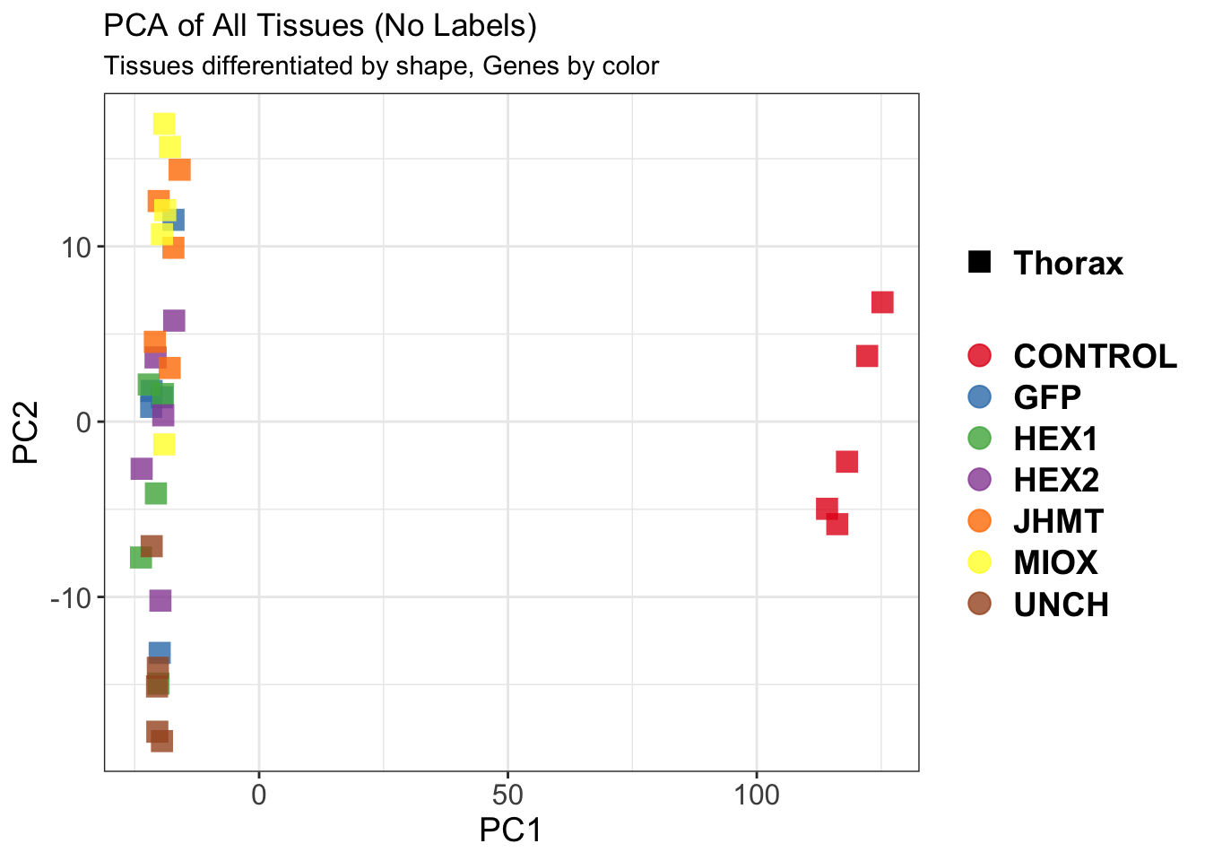
| Version | Author | Date |
|---|---|---|
| b540a1e | Maeva TECHER | 2025-02-27 |
$WithLabel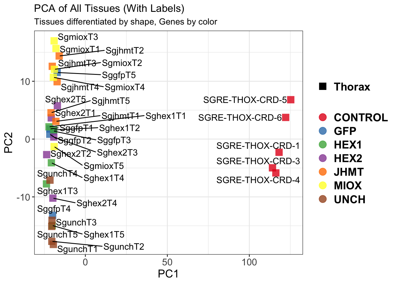
| Version | Author | Date |
|---|---|---|
| b540a1e | Maeva TECHER | 2025-02-27 |
The PCA plot shows clear distinction between tissue types, while gene silencing has a large variation within each tissue, and presents no distinct clear groupings for a single gene.
SVA
### SVA analysis to control for technical variation
dat <- counts(dds, normalized = TRUE)
idx <- rowMeans(dat) > 1
dat <- dat[idx, ]
mod <- model.matrix(~ Gene, colData(dds))
mod0 <- model.matrix(~ 1, colData(dds))
svseq <- svaseq(dat, mod, mod0)Number of significant surrogate variables is: 6
Iteration (out of 5 ):1 2 3 4 5 sva_plots <- create_sva_plots(svseq, dds, saveDir, intgroup = c("Tissue", "Gene"), max_sv = 6)
# Show stripcharts in the report
sva_plots$Stripcharts[[1]] # Show first stripchart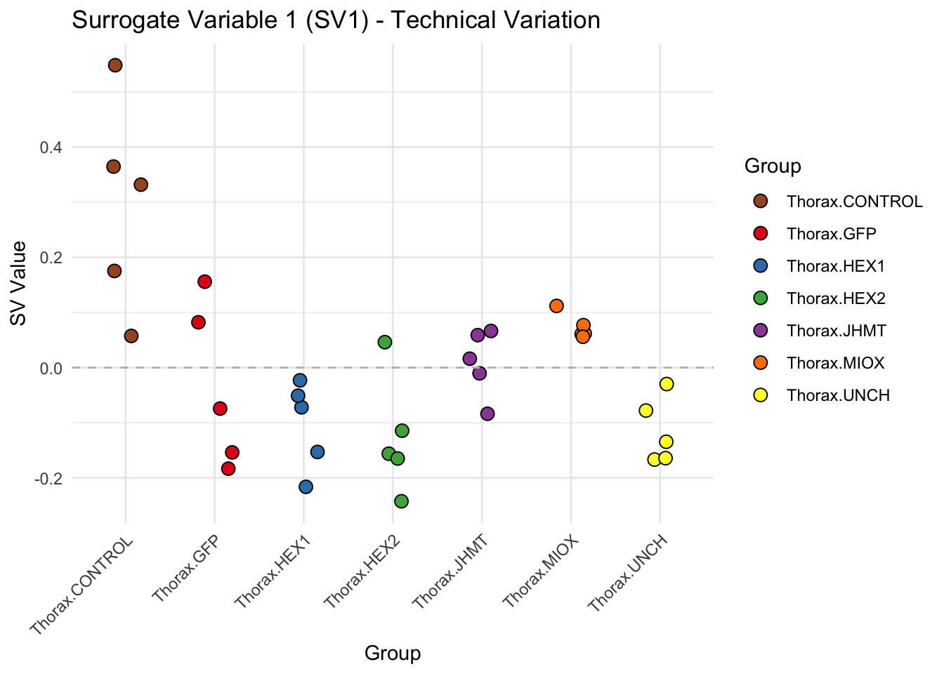
| Version | Author | Date |
|---|---|---|
| b540a1e | Maeva TECHER | 2025-02-27 |
sva_plots$Stripcharts[[2]] # Show second stripchart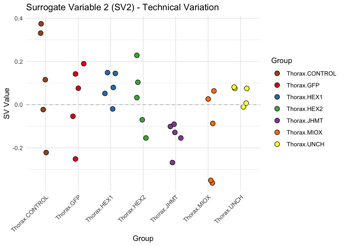
| Version | Author | Date |
|---|---|---|
| b540a1e | Maeva TECHER | 2025-02-27 |
sva_plots$Stripcharts[[3]] # Show third stripchart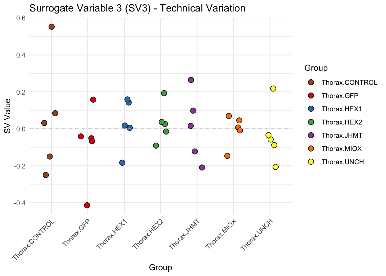
| Version | Author | Date |
|---|---|---|
| b540a1e | Maeva TECHER | 2025-02-27 |
sva_plots$Stripcharts[[4]] 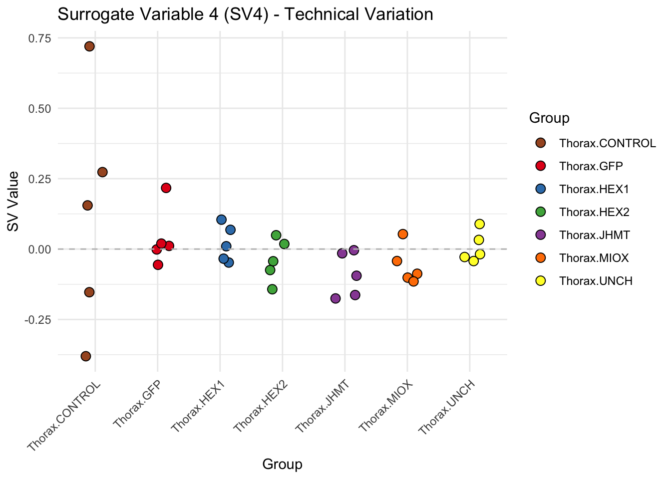
| Version | Author | Date |
|---|---|---|
| b540a1e | Maeva TECHER | 2025-02-27 |
sva_plots$Stripcharts[[5]] # Show third stripchart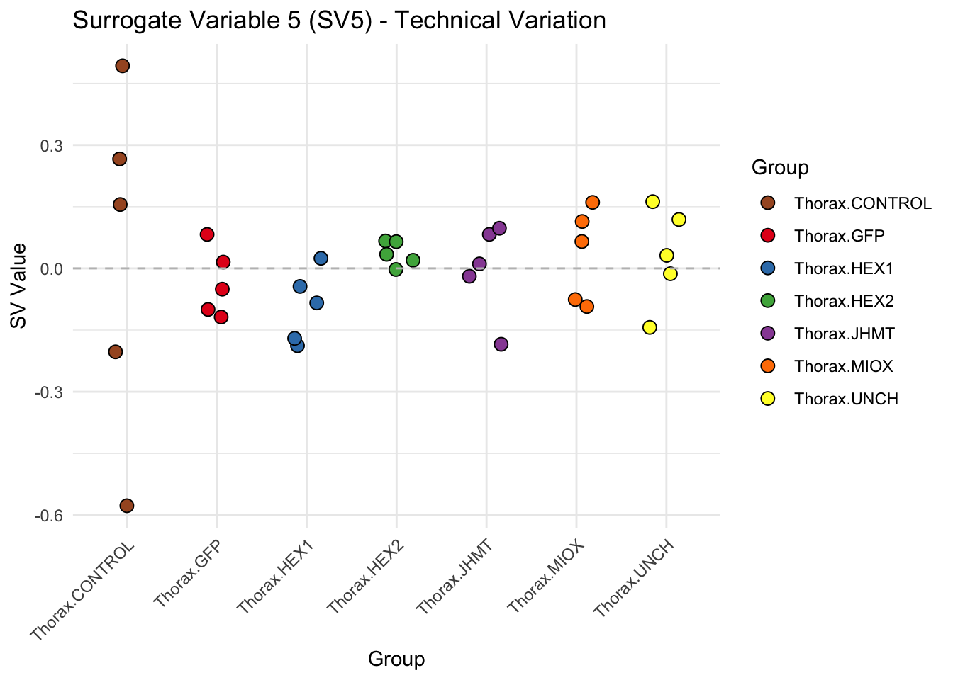
| Version | Author | Date |
|---|---|---|
| b540a1e | Maeva TECHER | 2025-02-27 |
sva_plots$Stripcharts[[6]] 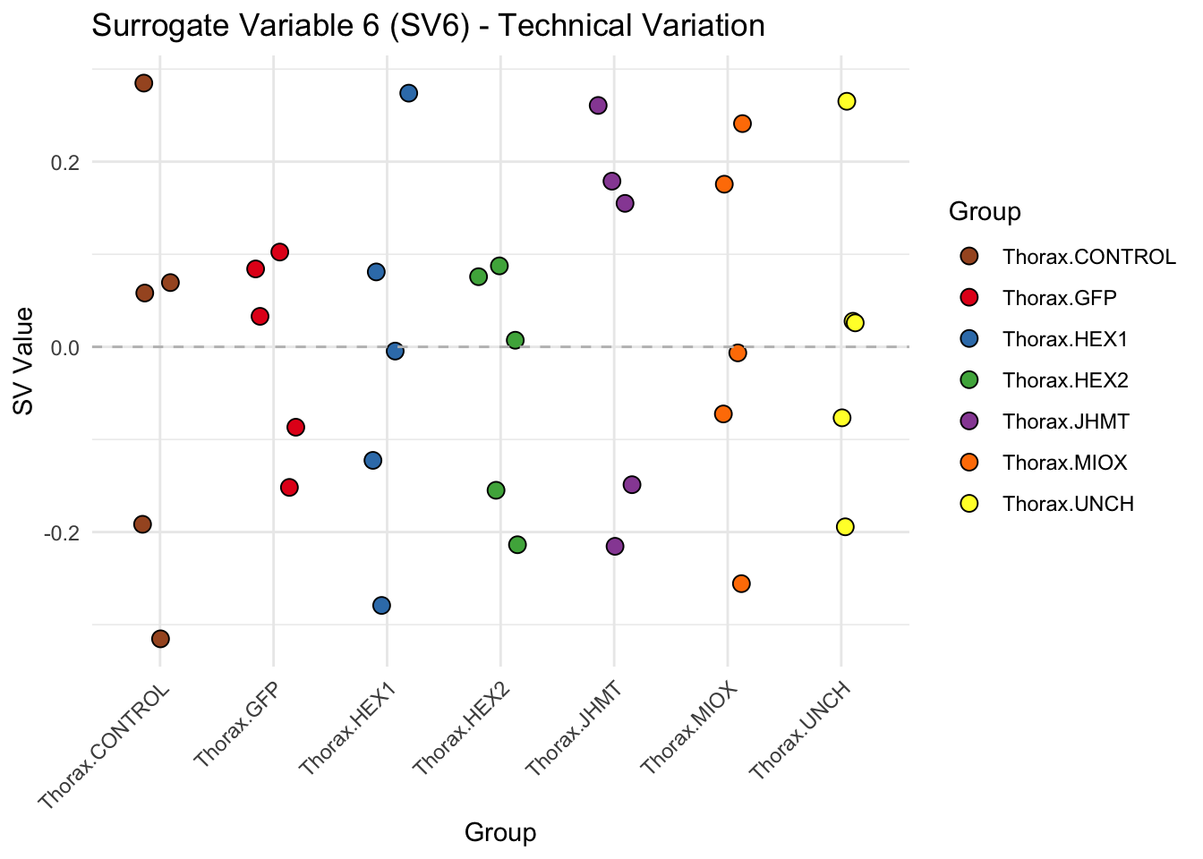
| Version | Author | Date |
|---|---|---|
| b540a1e | Maeva TECHER | 2025-02-27 |
# Show scatter plots in the report
sva_plots$ScatterPlots[["1_2"]] # Show SV1 vs SV2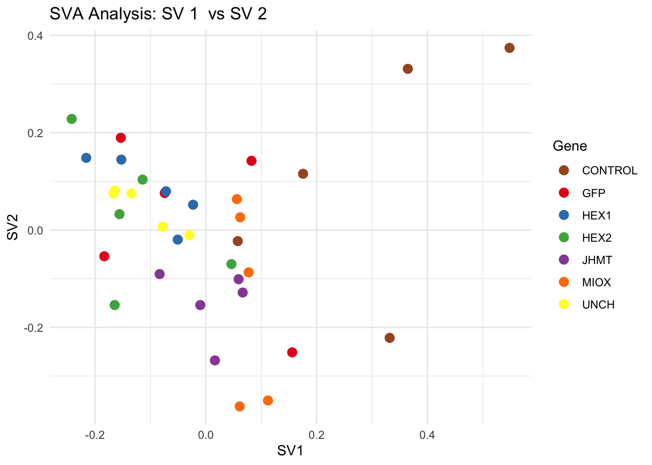
| Version | Author | Date |
|---|---|---|
| b540a1e | Maeva TECHER | 2025-02-27 |
sva_plots$ScatterPlots[["1_3"]] # Show SV1 vs SV3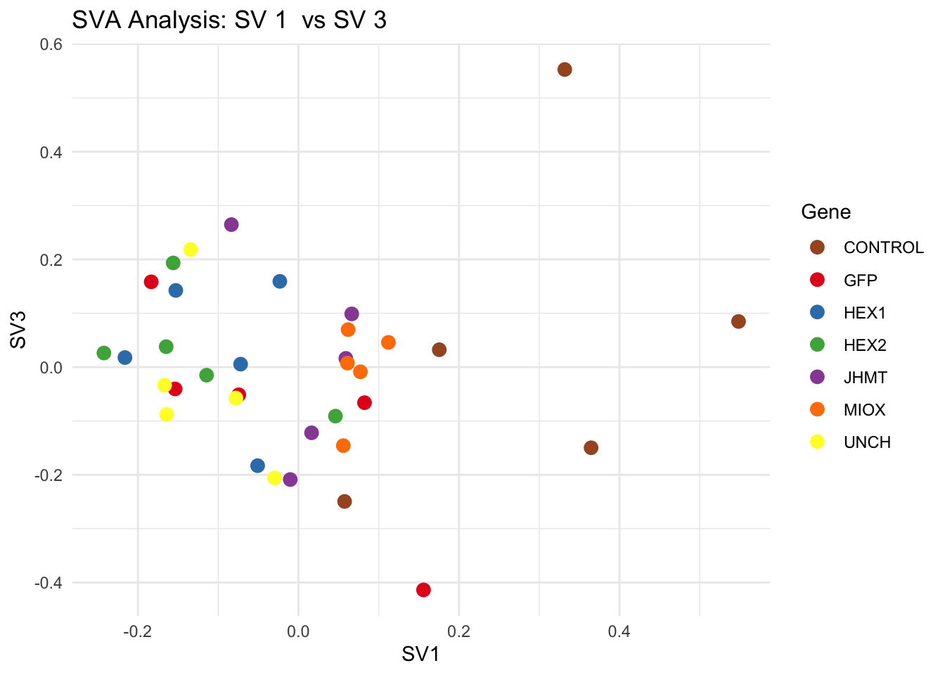
| Version | Author | Date |
|---|---|---|
| b540a1e | Maeva TECHER | 2025-02-27 |
sva_plots$ScatterPlots[["2_3"]] # Show SV2 vs SV3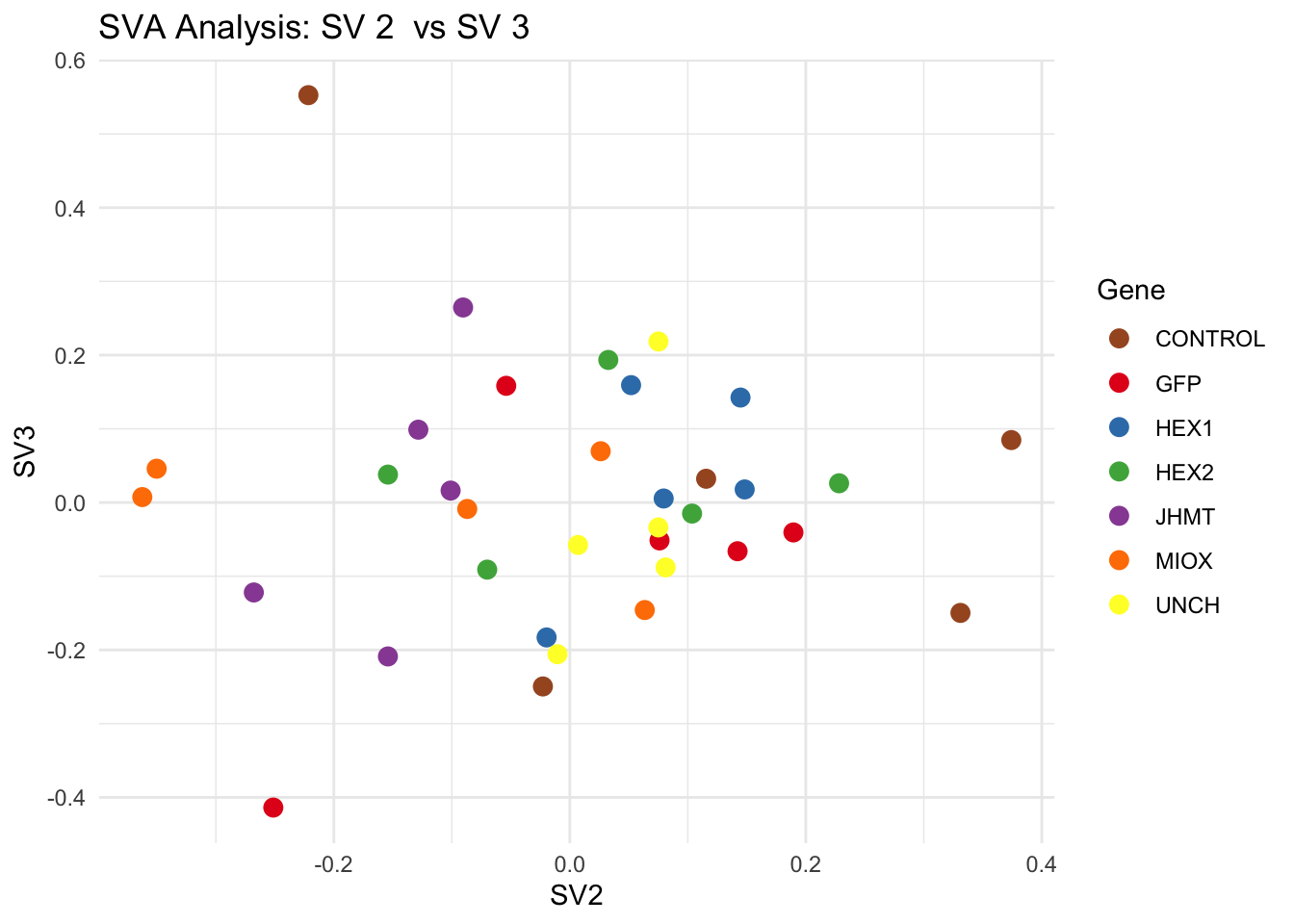
| Version | Author | Date |
|---|---|---|
| b540a1e | Maeva TECHER | 2025-02-27 |
SV1 is clearly showing an effect of tissue. We rerun the
DESeq2 model but this time including the surrogate variable
SV2 and SV3 as a covariates only, as we know that the modeled variation
is more likely explained by tissue and gene variation rather than batch
effects.
ddssva <- dds
ddssva$SV1 <- svseq$sv[,1]
ddssva$SV2 <- svseq$sv[,2]
ddssva$SV3 <- svseq$sv[,3]
ddssva$SV4 <- svseq$sv[,4]
ddssva$SV5 <- svseq$sv[,5]
ddssva$SV6 <- svseq$sv[,6]
design(ddssva) <- ~ SV1 + SV2 + SV3 + SV4 + SV5 + SV6 + Gene
ddssva$Gene <- relevel(ddssva$Gene, ref = "CONTROL")
smallestGroupSize <- 5
keep <- rowSums(counts(ddssva) >= 10) >= smallestGroupSize
ddssva <- ddssva[keep,]
ddssva <- DESeq(ddssva)
ddssva <- ddssva[which(mcols(ddssva)$betaConv),] # remove non converging rows
### Extract results
message("Available contrasts are: ", paste(resultsNames(ddssva), collapse = ", "))
hex1 <- results(ddssva, contrast = c("Gene", "HEX1", "CONTROL"), alpha = 0.05)
hex2 <- results(ddssva, contrast = c("Gene", "HEX2", "CONTROL"), alpha = 0.05)
jhmt <- results(ddssva, contrast = c("Gene", "JHMT", "CONTROL"), alpha = 0.05)
miox <- results(ddssva, contrast = c("Gene", "MIOX", "CONTROL"), alpha = 0.05)
unch <- results(ddssva, contrast = c("Gene", "UNCH", "CONTROL"), alpha = 0.05)
gfp <- results(ddssva, contrast = c("Gene", "GFP", "CONTROL"), alpha = 0.05)Volcano plots and Heatmaps
# Define contrast_sets
hex1_samples <- c("SGRE-THOX-CRD-1","SGRE-THOX-CRD-3","SGRE-THOX-CRD-4","SGRE-THOX-CRD-5",
"SGRE-THOX-CRD-6","SggfpT1","SggfpT2","SggfpT3","SggfpT4","SggfpT5",
"Sghex1T1","Sghex1T2","Sghex1T3","Sghex1T4","Sghex1T5")
hex2_samples <- c("SGRE-THOX-CRD-1","SGRE-THOX-CRD-3","SGRE-THOX-CRD-4","SGRE-THOX-CRD-5",
"SGRE-THOX-CRD-6","SggfpT1","SggfpT2","SggfpT3","SggfpT4","SggfpT5",
"Sghex2T1","Sghex2T2","Sghex2T3","Sghex2T4","Sghex2T5")
jhmt_samples <- c("SGRE-THOX-CRD-1","SGRE-THOX-CRD-3","SGRE-THOX-CRD-4","SGRE-THOX-CRD-5",
"SGRE-THOX-CRD-6","SggfpT1","SggfpT2","SggfpT3","SggfpT4","SggfpT5",
"SgjhmtT1","SgjhmtT2","SgjhmtT3","SgjhmtT4","SgjhmtT5")
miox_samples <- c("SGRE-THOX-CRD-1","SGRE-THOX-CRD-3","SGRE-THOX-CRD-4","SGRE-THOX-CRD-5",
"SGRE-THOX-CRD-6","SggfpT1","SggfpT2","SggfpT3","SggfpT4","SggfpT5",
"SgmioxT1","SgmioxT2","SgmioxT3","SgmioxT4","SgmioxT5")
unch_samples <- c("SGRE-THOX-CRD-1","SGRE-THOX-CRD-3","SGRE-THOX-CRD-4","SGRE-THOX-CRD-5",
"SGRE-THOX-CRD-6","SggfpT1","SggfpT2","SggfpT3","SggfpT4","SggfpT5",
"SgunchT1","SgunchT2","SgunchT3","SgunchT4","SgunchT5")
gfp_samples <- c("SGRE-THOX-CRD-1","SGRE-THOX-CRD-3","SGRE-THOX-CRD-4","SGRE-THOX-CRD-5",
"SGRE-THOX-CRD-6", "SggfpT1","SggfpT2","SggfpT3","SggfpT4","SggfpT5")
# Run full analysis
hex1_plots <- visualize_data_nopng(hex1, "HEX1_vs_CONTROL", hex1_samples)
hex2_plots <- visualize_data_nopng(hex2, "HEX2_vs_CONTROL", hex2_samples)
jhmt_plots <- visualize_data_nopng(jhmt, "JHMT_vs_CONTROL", jhmt_samples)
miox_plots <- visualize_data_nopng(miox, "MIOX_vs_CONTROL", miox_samples)
unch_plots <- visualize_data_nopng(unch, "UNCH_vs_CONTROL", unch_samples)
gfp_plots <- visualize_data_nopng(gfp, "GFP_vs_CONTROL", gfp_samples)
hex1_plots$volcano; hex1_plots$heatmap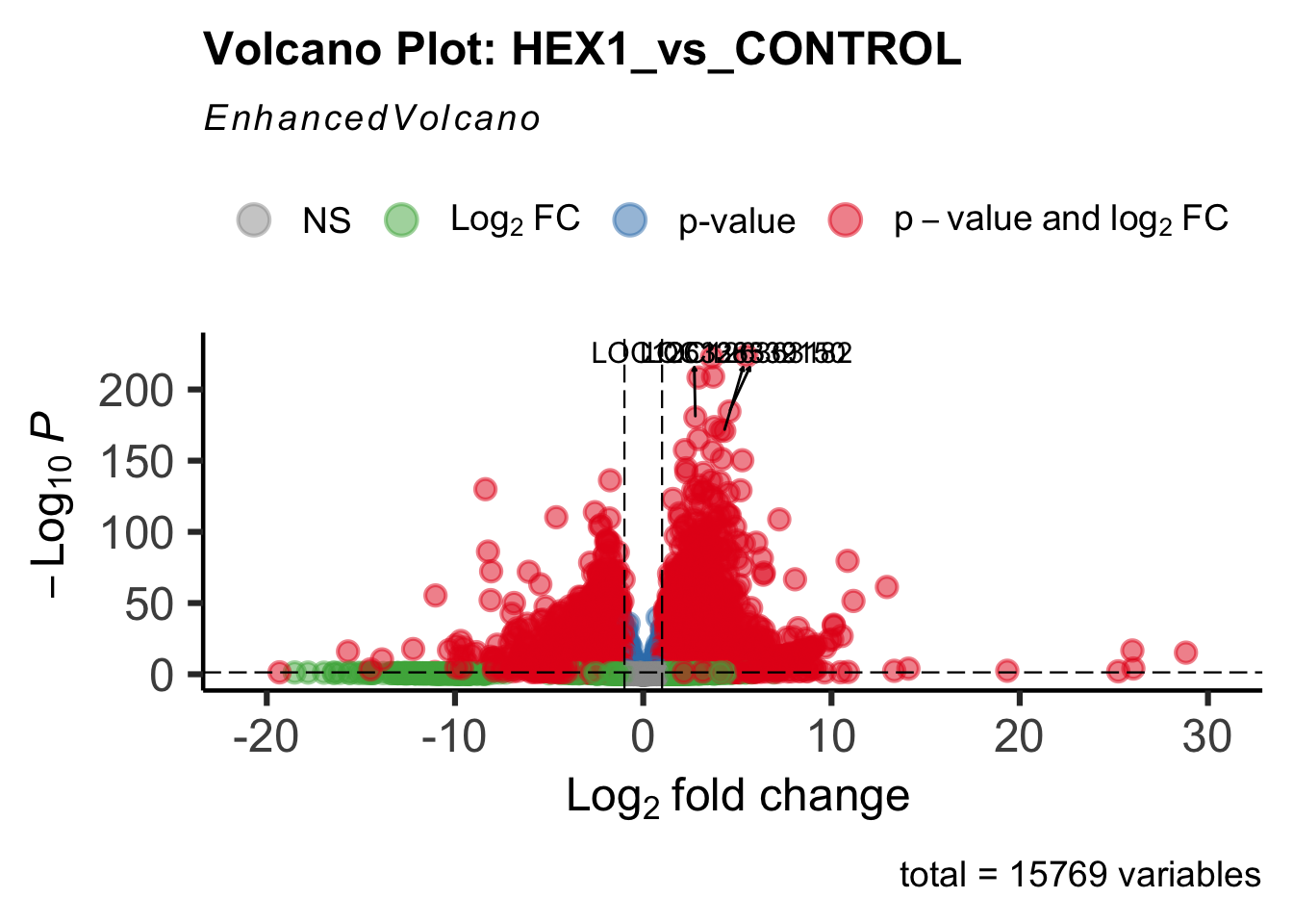
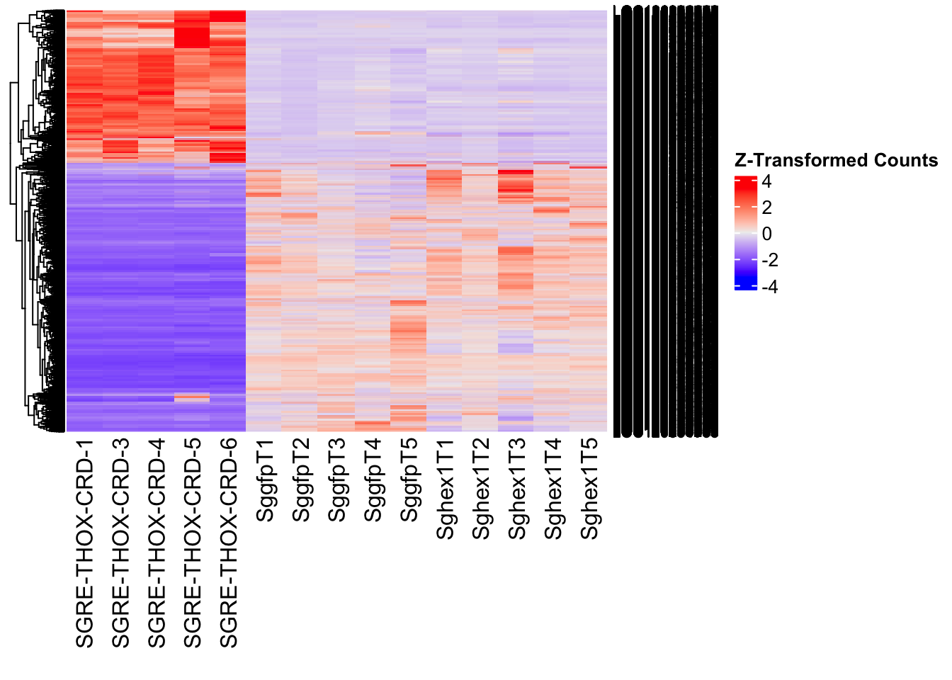
hex2_plots$volcano; hex2_plots$heatmap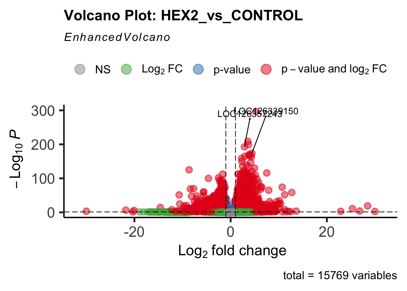
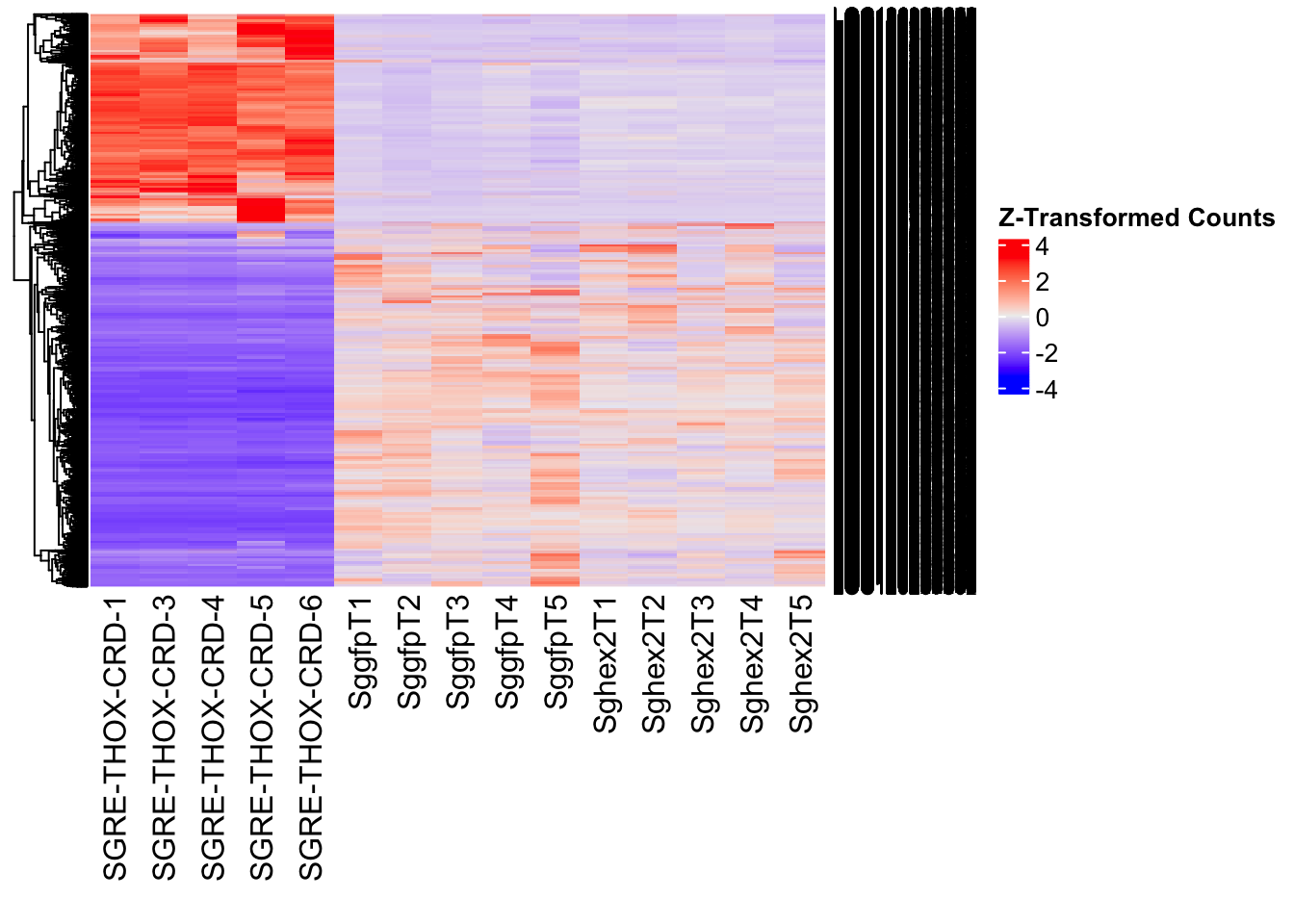
| Version | Author | Date |
|---|---|---|
| b540a1e | Maeva TECHER | 2025-02-27 |
jhmt_plots$volcano; jhmt_plots$heatmap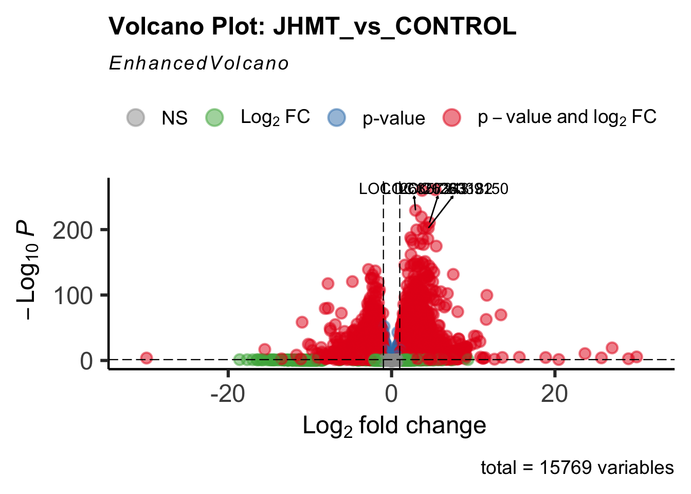
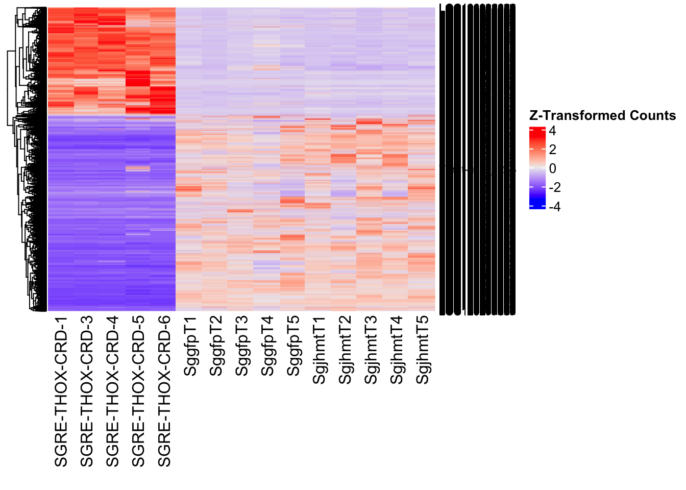
| Version | Author | Date |
|---|---|---|
| b540a1e | Maeva TECHER | 2025-02-27 |
miox_plots$volcano; miox_plots$heatmap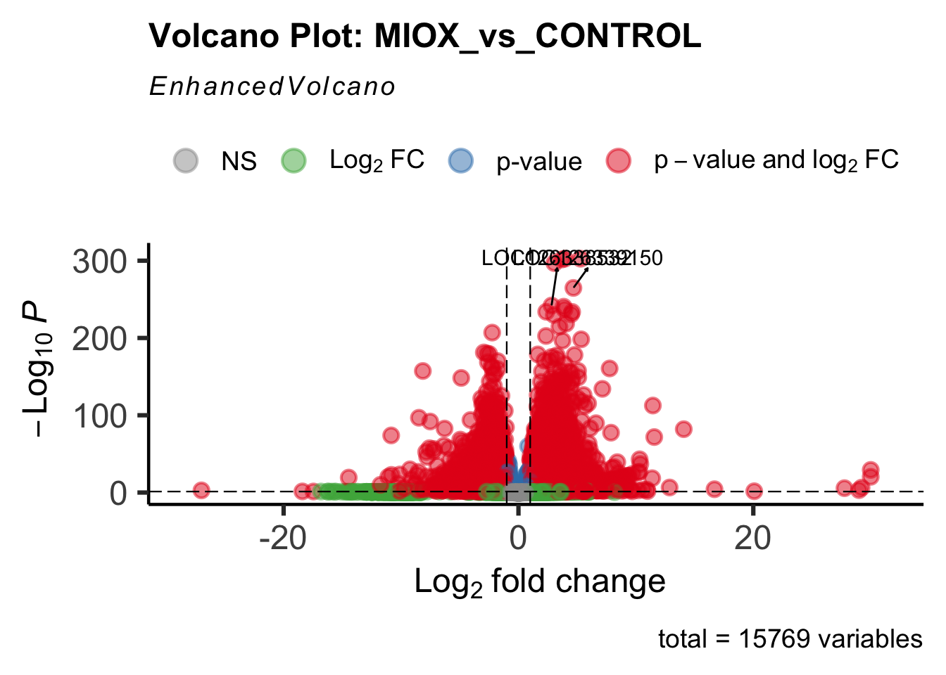
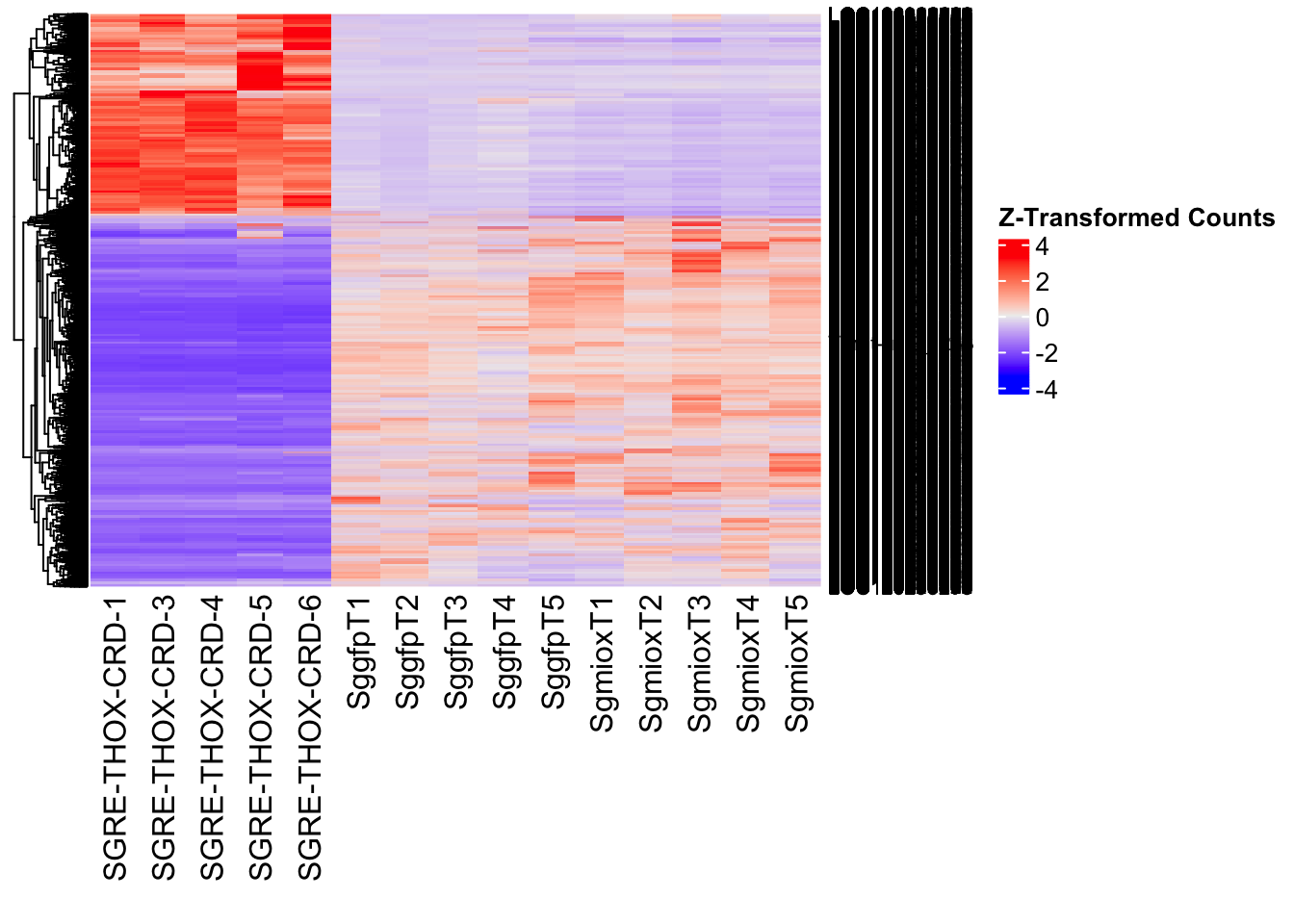
| Version | Author | Date |
|---|---|---|
| b540a1e | Maeva TECHER | 2025-02-27 |
unch_plots$volcano; unch_plots$heatmap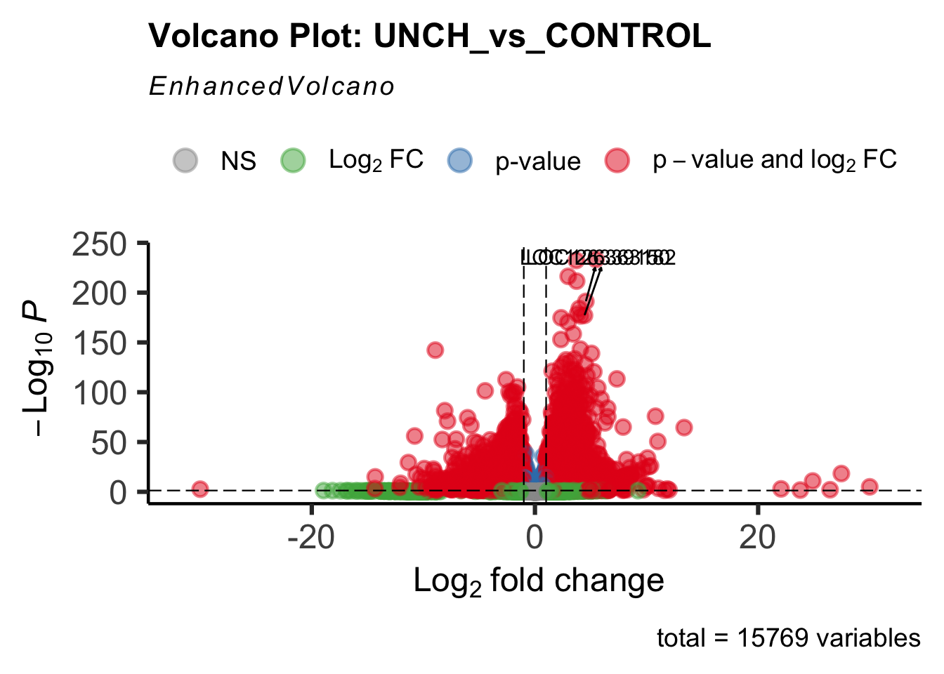
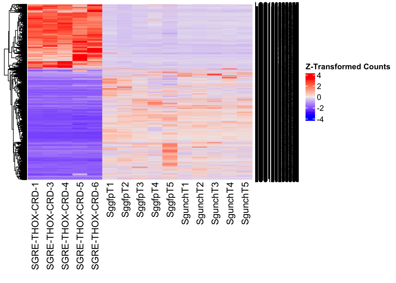
| Version | Author | Date |
|---|---|---|
| b540a1e | Maeva TECHER | 2025-02-27 |
gfp_plots$volcano; gfp_plots$heatmap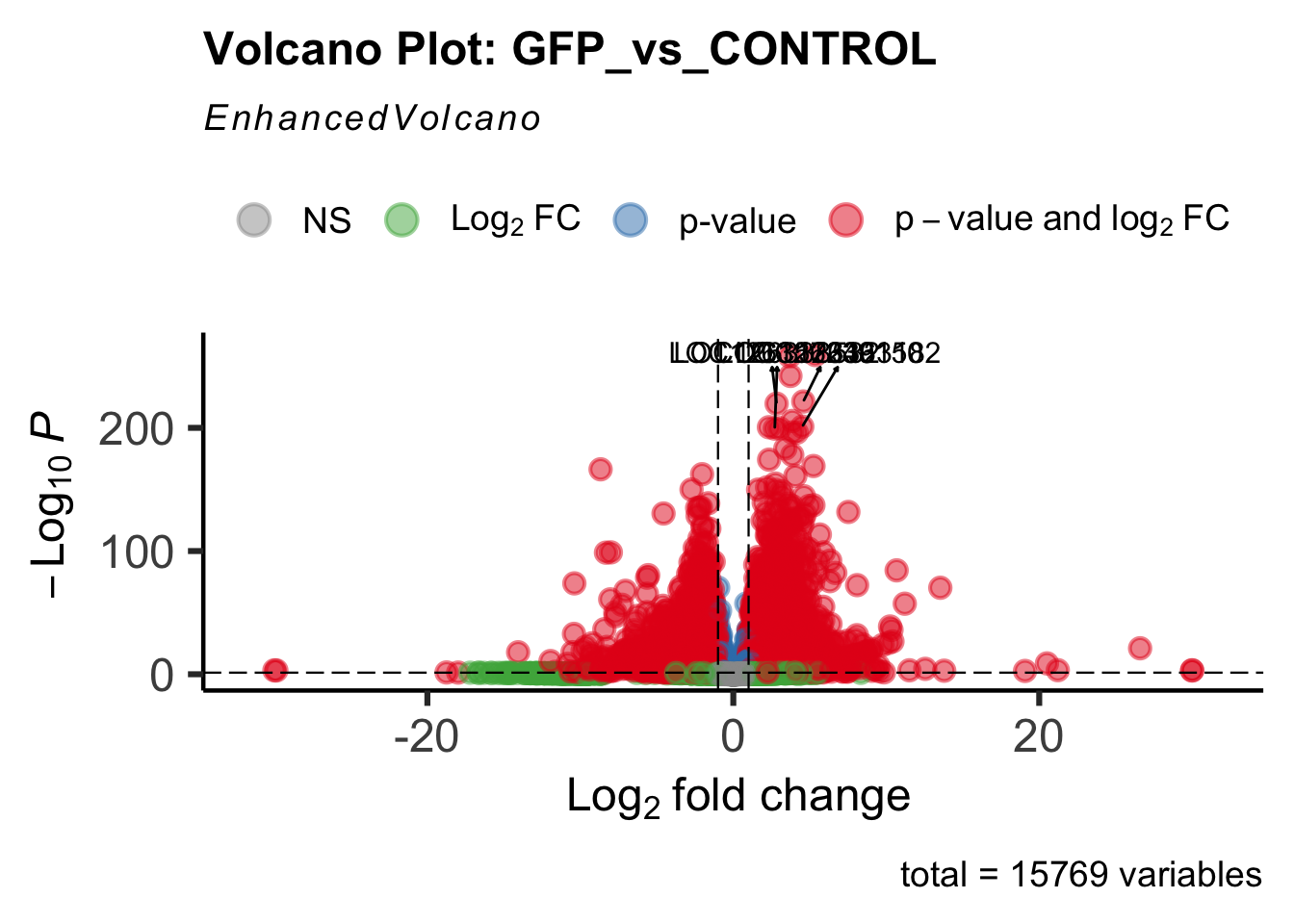
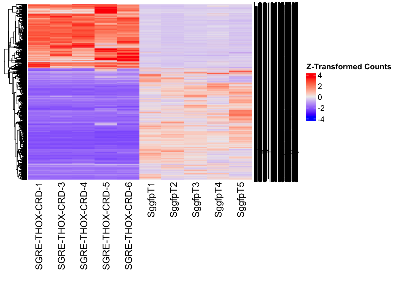
DEG tables
The following tables show the genes differentially expressed with at least an absolute log2fold change of > 1 considering Head tissues only. Considering GFP as the reference state, upregulated genes in knockdown treatment in red and downregulated genes in knockdown treatment in blue. You can search for a gene of interest by writting a LOCID or description in the search bar or sort by column.
# Generate tables for each contrast
table_hex1 <- generate_deg_table(ddssva, "Gene_HEX1_vs_CONTROL", allspecies_df)
out of 15769 with nonzero total read count
adjusted p-value < 0.05
LFC > 0 (up) : 6786, 43%
LFC < 0 (down) : 4354, 28%
outliers [1] : 0, 0%
low counts [2] : 0, 0%
(mean count < 3)
[1] see 'cooksCutoff' argument of ?results
[2] see 'independentFiltering' argument of ?resultsTotal DEGs p-value < 0.05 and absolute logFoldChange > 1: 8860LFC > 1 (up) : 5653 (63.8%)LFC < -1 (down) : 3207 (36.2%)table_hex1$kable_tabletable_hex2 <- generate_deg_table(ddssva, "Gene_HEX2_vs_CONTROL", allspecies_df)
out of 15769 with nonzero total read count
adjusted p-value < 0.05
LFC > 0 (up) : 6502, 41%
LFC < 0 (down) : 4314, 27%
outliers [1] : 0, 0%
low counts [2] : 0, 0%
(mean count < 3)
[1] see 'cooksCutoff' argument of ?results
[2] see 'independentFiltering' argument of ?resultsTotal DEGs p-value < 0.05 and absolute logFoldChange > 1: 8507LFC > 1 (up) : 5403 (63.51%)LFC < -1 (down) : 3104 (36.49%)table_hex2$kable_tabletable_jhmt <- generate_deg_table(ddssva, "Gene_JHMT_vs_CONTROL", allspecies_df)
out of 15769 with nonzero total read count
adjusted p-value < 0.05
LFC > 0 (up) : 7022, 45%
LFC < 0 (down) : 4439, 28%
outliers [1] : 0, 0%
low counts [2] : 0, 0%
(mean count < 3)
[1] see 'cooksCutoff' argument of ?results
[2] see 'independentFiltering' argument of ?resultsTotal DEGs p-value < 0.05 and absolute logFoldChange > 1: 9151LFC > 1 (up) : 5909 (64.57%)LFC < -1 (down) : 3242 (35.43%)table_jhmt$kable_tabletable_miox <- generate_deg_table(ddssva, "Gene_MIOX_vs_CONTROL", allspecies_df)
out of 15769 with nonzero total read count
adjusted p-value < 0.05
LFC > 0 (up) : 7277, 46%
LFC < 0 (down) : 4615, 29%
outliers [1] : 0, 0%
low counts [2] : 0, 0%
(mean count < 3)
[1] see 'cooksCutoff' argument of ?results
[2] see 'independentFiltering' argument of ?resultsTotal DEGs p-value < 0.05 and absolute logFoldChange > 1: 9376LFC > 1 (up) : 6050 (64.53%)LFC < -1 (down) : 3326 (35.47%)table_miox$kable_tabletable_unch <- generate_deg_table(ddssva, "Gene_UNCH_vs_CONTROL", allspecies_df)
out of 15769 with nonzero total read count
adjusted p-value < 0.05
LFC > 0 (up) : 6591, 42%
LFC < 0 (down) : 4391, 28%
outliers [1] : 0, 0%
low counts [2] : 0, 0%
(mean count < 3)
[1] see 'cooksCutoff' argument of ?results
[2] see 'independentFiltering' argument of ?resultsTotal DEGs p-value < 0.05 and absolute logFoldChange > 1: 8646LFC > 1 (up) : 5467 (63.23%)LFC < -1 (down) : 3179 (36.77%)table_unch$kable_tabletable_gfp <- generate_deg_table(ddssva, "Gene_GFP_vs_CONTROL", allspecies_df)
out of 15769 with nonzero total read count
adjusted p-value < 0.05
LFC > 0 (up) : 6989, 44%
LFC < 0 (down) : 4513, 29%
outliers [1] : 0, 0%
low counts [2] : 0, 0%
(mean count < 3)
[1] see 'cooksCutoff' argument of ?results
[2] see 'independentFiltering' argument of ?resultsTotal DEGs p-value < 0.05 and absolute logFoldChange > 1: 9075LFC > 1 (up) : 5779 (63.68%)LFC < -1 (down) : 3296 (36.32%)table_gfp$kable_tableSummary and Overlap
# Summarize DEGs for all contrasts
deg_summary <- bind_rows(
summarize_deg_counts(table_hex1, "HEX1 vs CONTROL"),
summarize_deg_counts(table_hex2, "HEX2 vs CONTROL"),
summarize_deg_counts(table_jhmt, "JHMT vs CONTROL"),
summarize_deg_counts(table_miox, "MIOX vs CONTROL"),
summarize_deg_counts(table_unch, "UNCH vs CONTROL"),
summarize_deg_counts(table_gfp, "GFP vs CONTROL")
)
# Display table using kable with styling
deg_summary %>%
kable("html", escape = FALSE, col.names = gsub("_", " ", names(.))) %>%
kable_styling("striped", full_width = TRUE) %>%
column_spec(2, color = "red", bold = TRUE) %>% # Upregulated in red
column_spec(3, color = "blue", bold = TRUE) %>% # Downregulated in blue
add_header_above(c("Summary of DEGs" = 3)) %>%
row_spec(0, bold = TRUE)| Contrast | Upregulated | Downregulated |
|---|---|---|
| HEX1 vs CONTROL | 5604 | 3186 |
| HEX2 vs CONTROL | 5338 | 3076 |
| JHMT vs CONTROL | 5852 | 3221 |
| MIOX vs CONTROL | 6011 | 3305 |
| UNCH vs CONTROL | 5411 | 3156 |
| GFP vs CONTROL | 5723 | 3276 |
# Define the list of RNAi contrasts
contrast_list <- c("HEX1_vs_CONTROL", "HEX2_vs_CONTROL", "JHMT_vs_CONTROL",
"MIOX_vs_CONTROL", "UNCH_vs_CONTROL", "GFP_vs_CONTROL")
# Initialize empty lists for storing Head-specific DEGs for each contrast
venn_data_up <- list()
venn_data_down <- list()
venn_data_all <- list()
# Function to load Head-specific DEGs for a given set of contrasts
load_deg_contrasts_head <- function(contrast_list) {
degs_up <- list()
degs_down <- list()
degs_all <- list()
for (contrast in contrast_list) {
deg_file <- file.path(workDir, "DEG_results/RNAi/Thorax_control/", contrast, paste0("DEG_sigresults_", contrast, ".csv"))
if (!file.exists(deg_file)) {
message(paste("File missing for contrast:", contrast))
next # Skip if the file doesn't exist
}
deg_data <- read.csv(deg_file, stringsAsFactors = FALSE)
# Convert row names to a column if necessary
if ("X" %in% colnames(deg_data)) {
colnames(deg_data)[colnames(deg_data) == "X"] <- "GeneID"
}
# Check if data is empty
if (nrow(deg_data) == 0) {
message(paste("No data for contrast:", contrast))
next
}
# Select significant DEGs (Up, Down, All)
degs_up[[contrast]] <- deg_data %>%
filter(padj < 0.05 & log2FoldChange >= 1) %>%
pull(GeneID) # Extract GeneID column
degs_down[[contrast]] <- deg_data %>%
filter(padj < 0.05 & log2FoldChange <= -1) %>%
pull(GeneID) # Extract GeneID column
degs_all[[contrast]] <- deg_data %>%
filter(padj < 0.05 & abs(log2FoldChange) >= 1) %>%
pull(GeneID) # Extract GeneID column
}
return(list(up = degs_up, down = degs_down, all = degs_all))
}
# Load DEG data for the defined contrasts (Head tissue only)
venn_data_contrasts <- load_deg_contrasts_head(contrast_list)
# Prepare the data for the Venn diagrams
venn_data_up <- venn_data_contrasts$up
venn_data_down <- venn_data_contrasts$down
venn_data_all <- venn_data_contrasts$all
# Display the Venn diagram and datatable for **Head Upregulated DEGs** across contrasts
display_ggvenn_plot(venn_data_up, "Venn Diagram of Thorax Upregulated DEGs - RNAi Contrasts")
# Display the Venn diagram and datatable for **Head Downregulated DEGs** across contrasts
display_ggvenn_plot(venn_data_down, "Venn Diagram of Thorax Downregulated DEGs - RNAi Contrasts")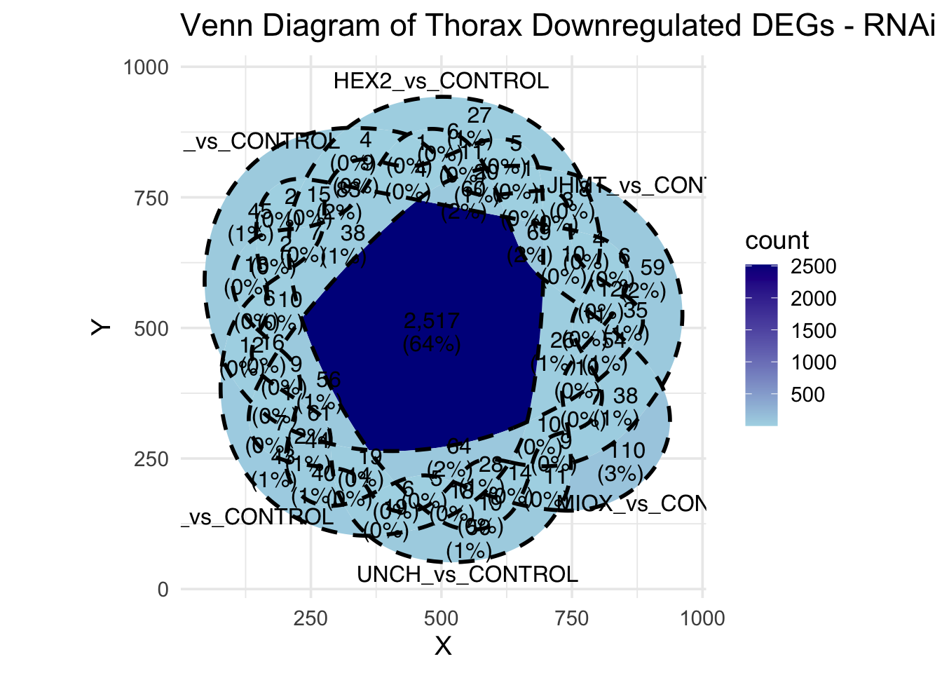
# Display the Venn diagram and datatable for **All Significant DEGs in Head Tissue**
display_ggvenn_plot(venn_data_all, "Venn Diagram of All Significant DEGs in Thorax Tissue - RNAi Contrasts")
# Run the UpSet plot for Head Upregulated DEGs
display_upset_plot(venn_data_up, "UpSet Plot of Thorax Upregulated DEGs - RNAi Contrasts")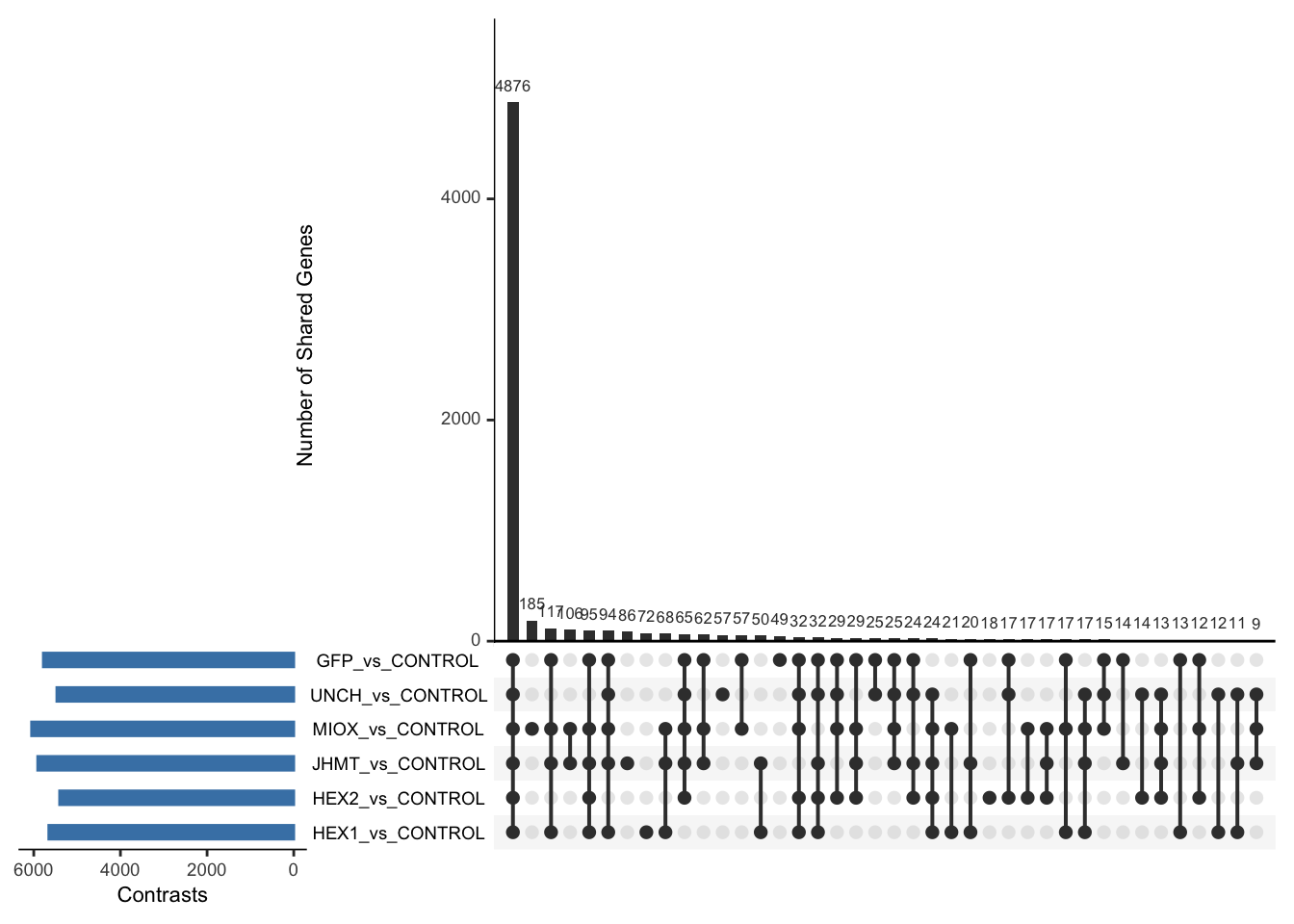
# Run the UpSet plot for Head Downregulated DEGs
display_upset_plot(venn_data_down, "UpSet Plot of Thorax Downregulated DEGs - RNAi Contrasts")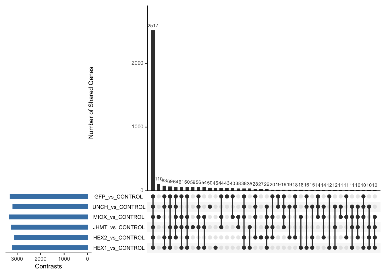
# Run the UpSet plot for Head Upregulated DEGs
display_upset_plot(venn_data_all, "UpSet Plot of All Significant DEGs in Thorax Tissue - RNAi Contrasts")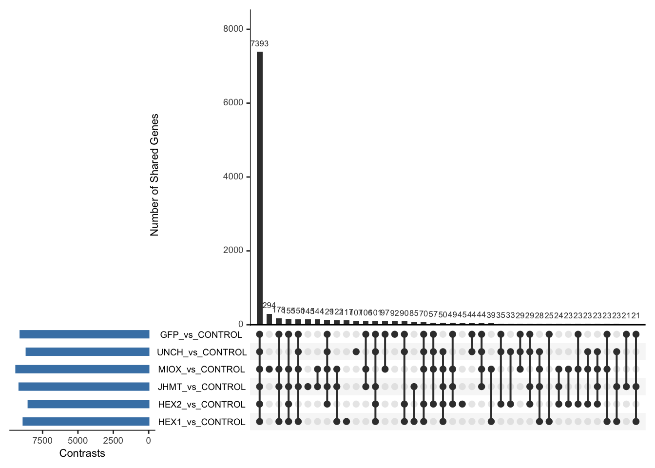
Excluding rRNA
All tissue together
Minor changes here are made compared to the DESeq2
results regarding the importation of samples to transform into a
matrix.
Sample names are structured as follow: {Sg}{gene}{#} {Sg} = Schistocerca gregaria {gene} = gene abbreviation gfp, hex1, hex2, jhmt, miox and unch H/T{#} = biological replicate
saveDir <- paste0(workDir,"/DEG_results/RNAi/All_control_no_rRNA")
dir.create(saveDir)
### Prepare Sample CSV file #####
samples <- read.delim(file.path(workDir, "list/RNAi/All_RNAi_noninjectedsample_list.csv"), sep = ",", row.names = 1, header = TRUE)
files <- file.path(workDir, "readcounts/RNAi/", samples$Tissue, samples$Filename)
names(files) <- row.names(samples)
if (all(file.exists(files))) {
message("All the files exist!")
} else {
warning("Some files are missing!")
}All the files exist!### **Standardized Count Matrix Creation**
# Extract all gene lists first
gene_lists <- map(files, function(sample) {
fread(sample, sep = "\t", header = FALSE)[, 1] # Extract Gene IDs (column 1)
})
# Get a unique set of all gene IDs across all samples
all_genes <- unique(unlist(gene_lists))
# Create a named list to store count data with standardized rows
cts_list <- map(files, function(sample) {
data_count <- fread(sample, sep = "\t", header = FALSE)
col_name <- gsub("_counts.txt", "", basename(sample)) # Clean sample name
# Convert to data frame with correct column names
data_count <- setNames(data.frame(data_count[, 1:2]), c("GeneID", col_name))
# Ensure all gene IDs are present (fill missing values with 0)
data_count <- full_join(data.frame(GeneID = all_genes), data_count, by = "GeneID") %>%
mutate(across(where(is.numeric), ~ replace_na(., 0))) # Fill NA with 0
return(data_count)
})
# Merge all samples based on GeneID
cts <- reduce(cts_list, full_join, by = "GeneID")
# Convert to matrix for DESeq2
cts_matrix <- as.matrix(cts[, -1]) # Remove GeneID column for count matrix
rownames(cts_matrix) <- cts$GeneID # Set GeneID as rownames
rm(cts_list) # Free memoryWhile for bulk RNAseq on head and thorax for all species, the DEGs model was made between isolated and crowded individuals (with isolated as the reference state), here, the DEG analysis will be carried between GFP knock-down nymphs (as reference state) vs Hexamerins / Juvenile Hormones / Inositol / Uncharacterized proteins.
### Build DESeq2 Object
dds <- DESeqDataSetFromMatrix(countData = cts_matrix,
colData = samples,
design = ~ Gene)
dds$Gene <- relevel(dds$Gene, ref = "CONTROL")
smallestGroupSize <- 5
keep <- rowSums(counts(dds) >= 10) >= smallestGroupSize
dds <- dds[keep,]
loci_to_exclude <- readLines(file.path(workDir, "list/excluded_loci/gregaria_rrna_list.txt"))
dds <- dds[!(rownames(dds) %in% loci_to_exclude), ]
dds <- DESeq(dds)Normalization and PCA
# Plot PCA and investigate quality metrics
vsd <- vst(dds, blind = TRUE)
# Perform PCA
pca_data <- plotPCA(vsd, intgroup = c("Tissue", "Gene"), returnData = TRUE)
# Define colors for genes (slightly transparent) and shapes for tissues
gene_colors <- scale_color_manual(values = alpha(brewer.pal(n = length(unique(pca_data$Gene)), name = "Set1"), 0.8)) # Points are transparent
tissue_shapes <- scale_shape_manual(values = seq(15, 15 + length(unique(pca_data$Tissue))))
# **PCA without labels**
p_pca_nolabel <- ggplot(pca_data, aes(x = PC1, y = PC2, color = Gene, shape = Tissue)) +
geom_point(size = 4) +
gene_colors +
tissue_shapes +
theme_bw() +
theme(legend.title = element_blank(),
legend.text = element_text(face = "bold", size = 14),
axis.text = element_text(size = 12),
axis.title = element_text(size = 14)) +
ggtitle("PCA of All Tissues (No Labels)", subtitle = "Tissues differentiated by shape, Genes by color")
# Save PCA without labels
ggsave(paste0(saveDir, "/PCA_Tissue_Gene_NoLabel.png"), plot = p_pca_nolabel, width = 10, height = 10, dpi = 600, device = "png")
# **PCA with labels**
p_pca_label <- ggplot(pca_data, aes(x = PC1, y = PC2, color = Gene, shape = Tissue)) +
geom_point(size = 4) +
geom_text_repel(aes(label = name), size = 4, color = "black", max.overlaps = 20) + # Labels are fully visible
gene_colors +
tissue_shapes +
theme_bw() +
theme(legend.title = element_blank(),
legend.text = element_text(face = "bold", size = 14),
axis.text = element_text(size = 12),
axis.title = element_text(size = 14)) +
ggtitle("PCA of All Tissues (With Labels)", subtitle = "Tissues differentiated by shape, Genes by color")
# Save PCA with labels
ggsave(paste0(saveDir, "/PCA_Tissue_Gene_Label.png"), plot = p_pca_label, width = 10, height = 10, dpi = 600, device = "png")
# **Return plots for knitr/RMarkdown**
list(NoLabel = p_pca_nolabel, WithLabel = p_pca_label)$NoLabel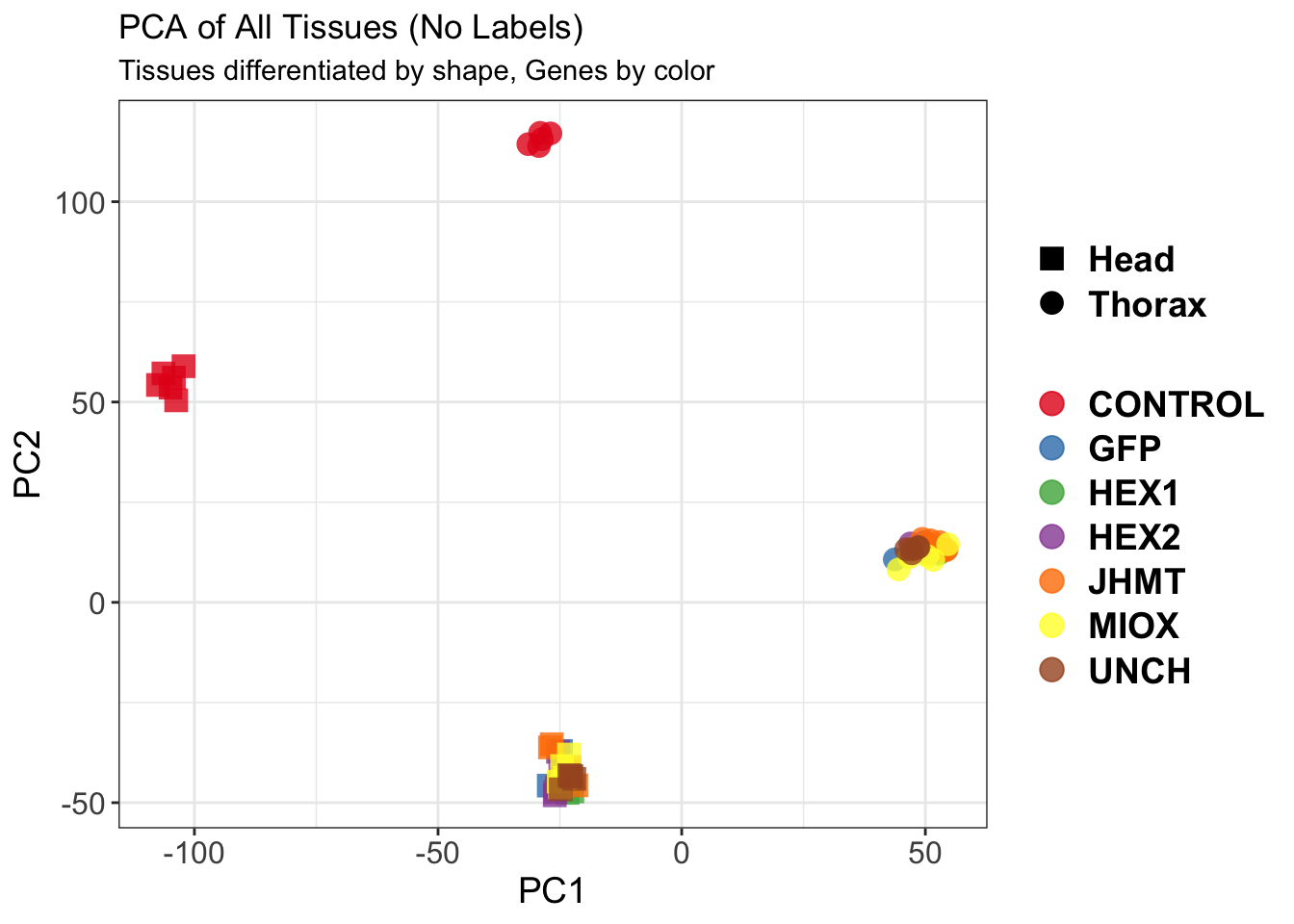
| Version | Author | Date |
|---|---|---|
| b540a1e | Maeva TECHER | 2025-02-27 |
$WithLabel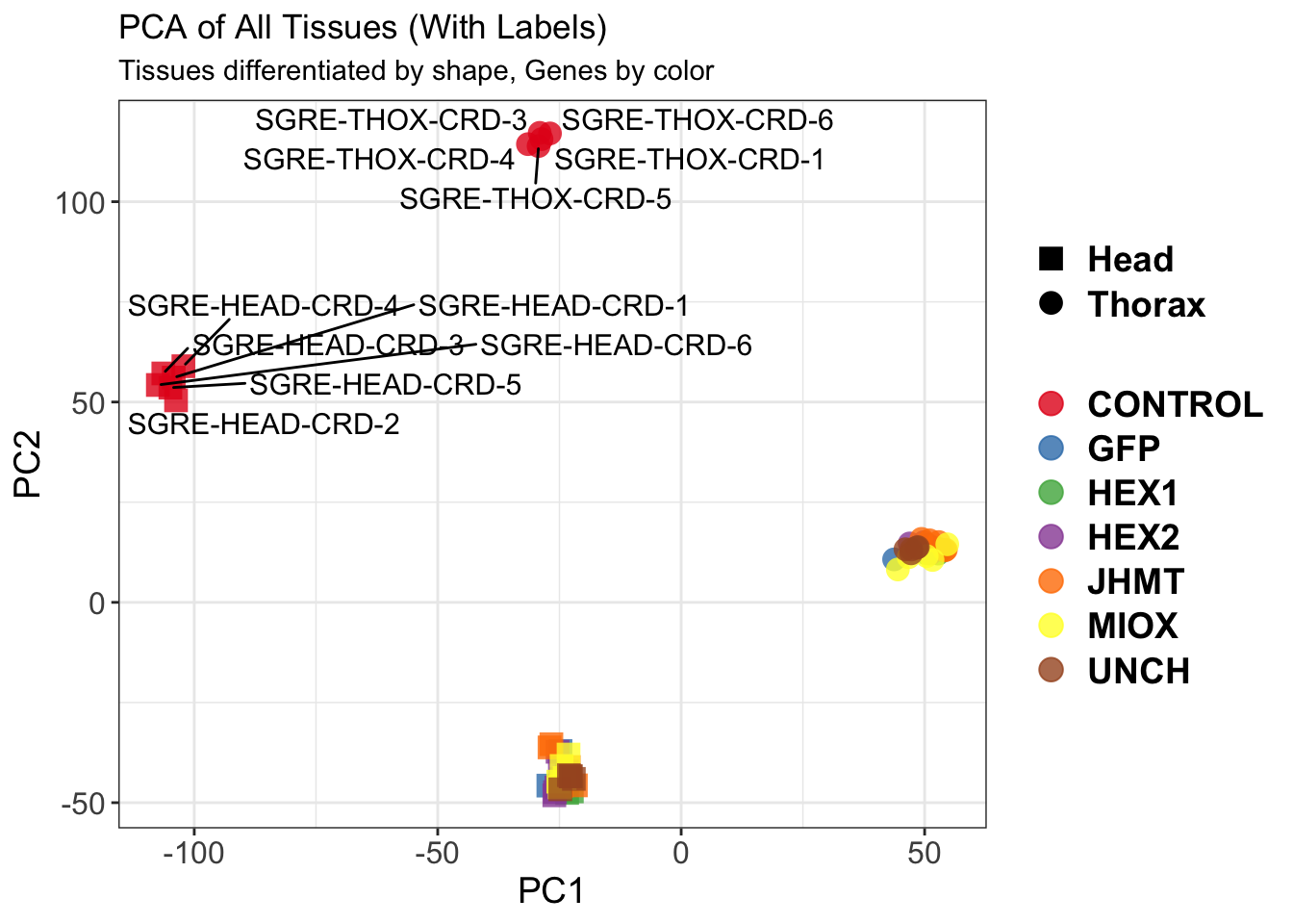
| Version | Author | Date |
|---|---|---|
| b540a1e | Maeva TECHER | 2025-02-27 |
The PCA plot shows clear distinction between tissue types, while gene silencing has a large variation within each tissue, and presents no distinct clear groupings for a single gene.
SVA
### SVA analysis to control for technical variation
dat <- counts(dds, normalized = TRUE)
idx <- rowMeans(dat) > 1
dat <- dat[idx, ]
mod <- model.matrix(~ Gene, colData(dds))
mod0 <- model.matrix(~ 1, colData(dds))
svseq <- svaseq(dat, mod, mod0)Number of significant surrogate variables is: 3
Iteration (out of 5 ):1 2 3 4 5 sva_plots <- create_sva_plots(svseq, dds, saveDir, intgroup = c("Tissue", "Gene"), max_sv = 3)
# Show stripcharts in the report
sva_plots$Stripcharts[[1]] # Show first stripchart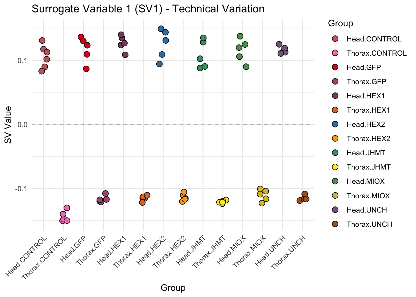
| Version | Author | Date |
|---|---|---|
| b540a1e | Maeva TECHER | 2025-02-27 |
sva_plots$Stripcharts[[2]] # Show second stripchart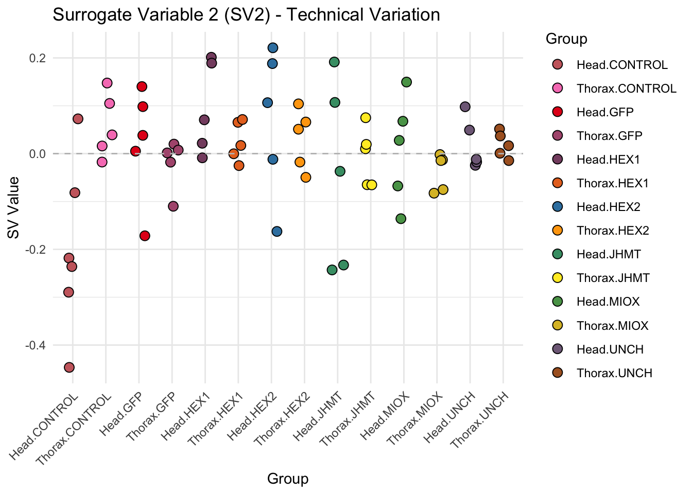
| Version | Author | Date |
|---|---|---|
| b540a1e | Maeva TECHER | 2025-02-27 |
sva_plots$Stripcharts[[3]] # Show third stripchart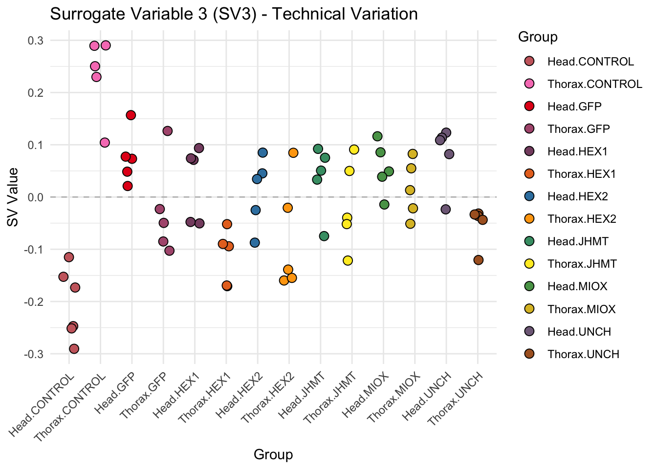
| Version | Author | Date |
|---|---|---|
| b540a1e | Maeva TECHER | 2025-02-27 |
# Show scatter plots in the report
sva_plots$ScatterPlots[["1_2"]] # Show SV1 vs SV2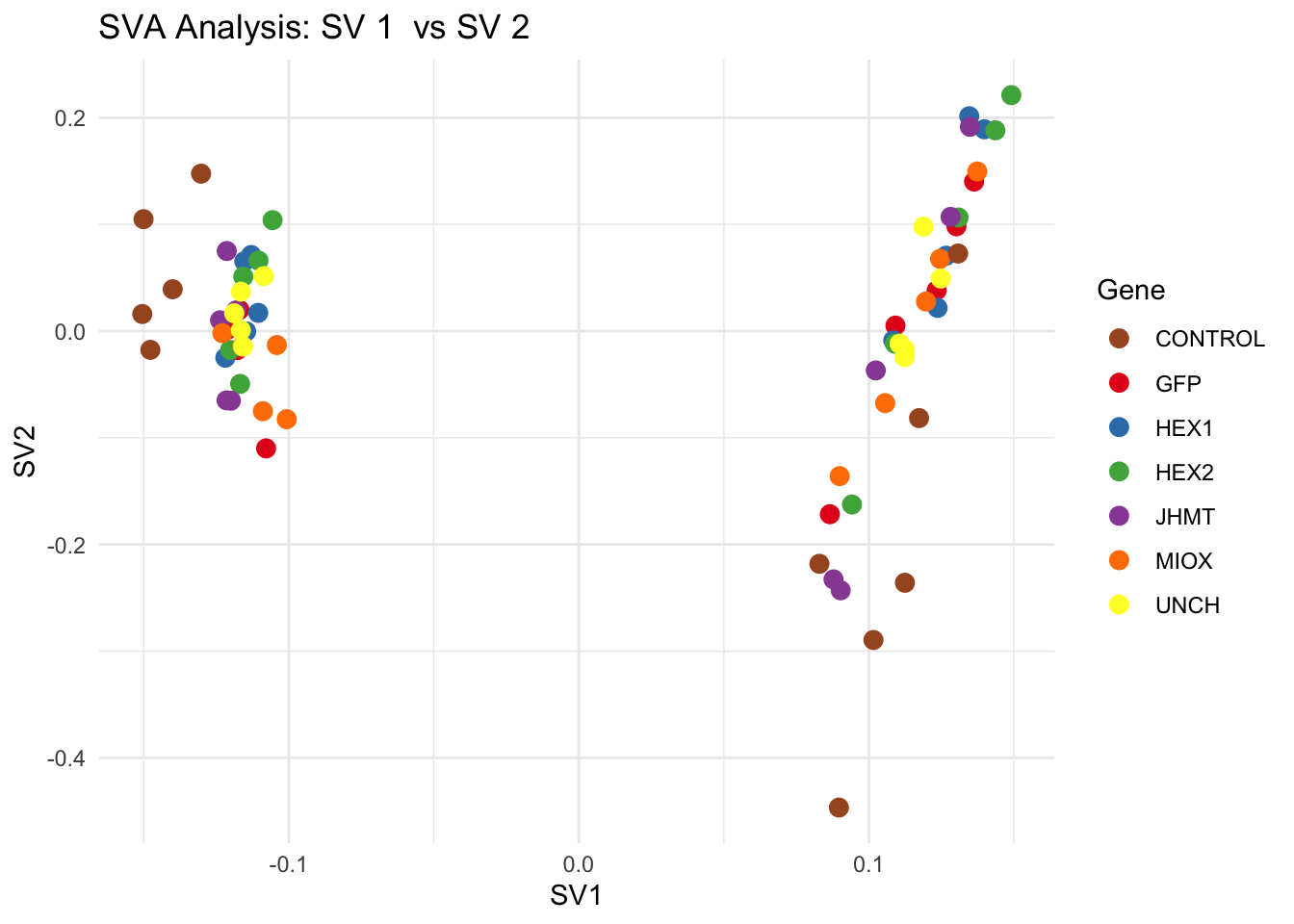
| Version | Author | Date |
|---|---|---|
| b540a1e | Maeva TECHER | 2025-02-27 |
sva_plots$ScatterPlots[["1_3"]] # Show SV1 vs SV3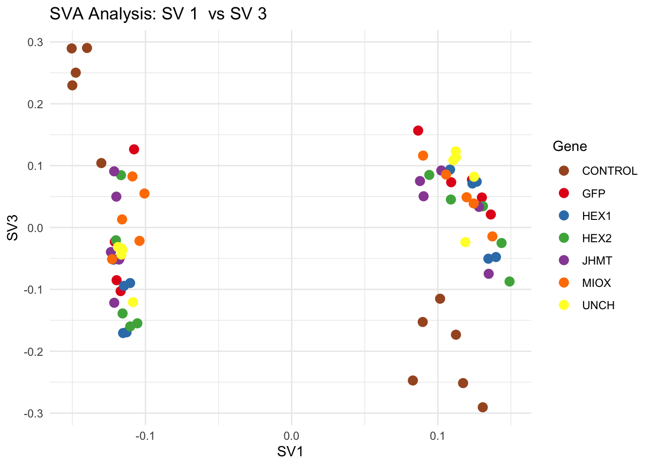
| Version | Author | Date |
|---|---|---|
| b540a1e | Maeva TECHER | 2025-02-27 |
sva_plots$ScatterPlots[["2_3"]] # Show SV2 vs SV3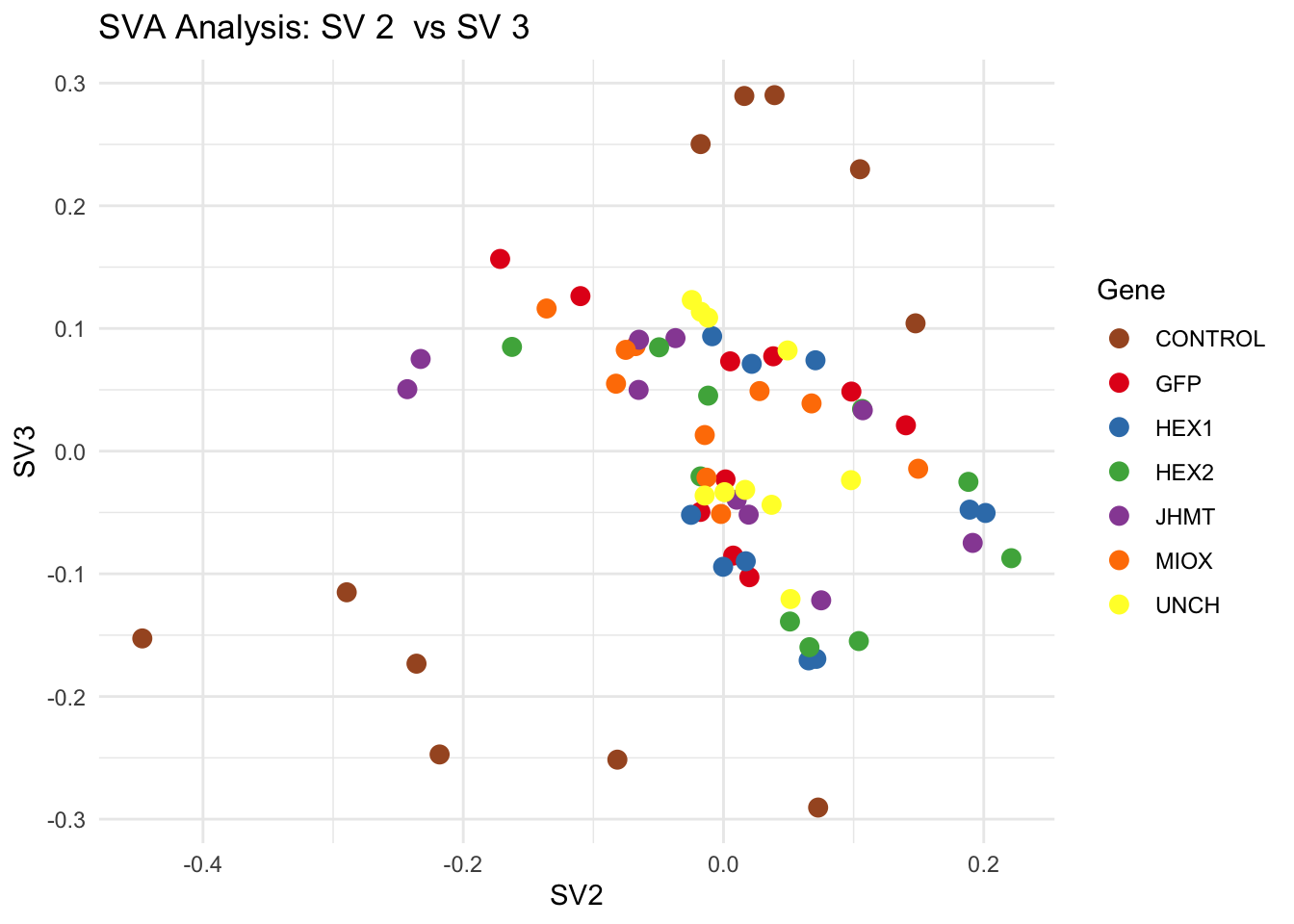
| Version | Author | Date |
|---|---|---|
| b540a1e | Maeva TECHER | 2025-02-27 |
SV1 is clearly showing an effect of tissue. We rerun the
DESeq2 model but this time including the surrogate variable
SV2 and SV3 as a covariates only, as we know that the modeled variation
is more likely explained by tissue and gene variation rather than batch
effects.
ddssva <- dds
ddssva$SV2 <- svseq$sv[,2]
ddssva$SV3 <- svseq$sv[,3]
design(ddssva) <- ~ SV2 + SV3 + Gene
ddssva$Gene <- relevel(ddssva$Gene, ref = "CONTROL")
smallestGroupSize <- 5
keep <- rowSums(counts(ddssva) >= 10) >= smallestGroupSize
ddssva <- ddssva[keep,]
ddssva <- DESeq(ddssva)
ddssva <- ddssva[which(mcols(ddssva)$betaConv),] # remove non converging rows
### Extract results
message("Available contrasts are: ", paste(resultsNames(ddssva), collapse = ", "))
hex1 <- results(ddssva, contrast = c("Gene", "HEX1", "CONTROL"), alpha = 0.05)
hex2 <- results(ddssva, contrast = c("Gene", "HEX2", "CONTROL"), alpha = 0.05)
jhmt <- results(ddssva, contrast = c("Gene", "JHMT", "CONTROL"), alpha = 0.05)
miox <- results(ddssva, contrast = c("Gene", "MIOX", "CONTROL"), alpha = 0.05)
unch <- results(ddssva, contrast = c("Gene", "UNCH", "CONTROL"), alpha = 0.05)
gfp <- results(ddssva, contrast = c("Gene", "GFP", "CONTROL"), alpha = 0.05)Volcano plots and Heatmaps
# Define contrast_sets
hex1_samples <- c("SGRE-HEAD-CRD-1","SGRE-HEAD-CRD-2","SGRE-HEAD-CRD-3","SGRE-HEAD-CRD-4","SGRE-HEAD-CRD-5",
"SGRE-HEAD-CRD-6","SggfpH1","SggfpH2","SggfpH3","SggfpH4","SggfpH5",
"Sghex1H1","Sghex1H2","Sghex1H3","Sghex1H4","Sghex1H5",
"SGRE-THOX-CRD-1","SGRE-THOX-CRD-3","SGRE-THOX-CRD-4","SGRE-THOX-CRD-5",
"SGRE-THOX-CRD-6","SggfpT1","SggfpT2","SggfpT3","SggfpT4","SggfpT5",
"Sghex1T1","Sghex1T2","Sghex1T3","Sghex1T4","Sghex1T5")
hex2_samples <- c("SGRE-HEAD-CRD-1","SGRE-HEAD-CRD-2","SGRE-HEAD-CRD-3","SGRE-HEAD-CRD-4","SGRE-HEAD-CRD-5",
"SGRE-HEAD-CRD-6","SggfpH1","SggfpH2","SggfpH3","SggfpH4","SggfpH5",
"Sghex2H1","Sghex2H2","Sghex2H3","Sghex2H4","Sghex2H5",
"SGRE-THOX-CRD-1","SGRE-THOX-CRD-3","SGRE-THOX-CRD-4","SGRE-THOX-CRD-5",
"SGRE-THOX-CRD-6","SggfpT1","SggfpT2","SggfpT3","SggfpT4","SggfpT5",
"Sghex2T1","Sghex2T2","Sghex2T3","Sghex2T4","Sghex2T5")
jhmt_samples <- c("SGRE-HEAD-CRD-1","SGRE-HEAD-CRD-2","SGRE-HEAD-CRD-3","SGRE-HEAD-CRD-4","SGRE-HEAD-CRD-5",
"SGRE-HEAD-CRD-6","SggfpH1","SggfpH2","SggfpH3","SggfpH4","SggfpH5",
"SgjhmtH1","SgjhmtH2","SgjhmtH3","SgjhmtH4","SgjhmtH5",
"SGRE-THOX-CRD-1","SGRE-THOX-CRD-3","SGRE-THOX-CRD-4","SGRE-THOX-CRD-5",
"SGRE-THOX-CRD-6","SggfpT1","SggfpT2","SggfpT3","SggfpT4","SggfpT5",
"SgjhmtT1","SgjhmtT2","SgjhmtT3","SgjhmtT4","SgjhmtT5")
miox_samples <- c("SGRE-HEAD-CRD-1","SGRE-HEAD-CRD-2","SGRE-HEAD-CRD-3","SGRE-HEAD-CRD-4","SGRE-HEAD-CRD-5",
"SGRE-HEAD-CRD-6","SggfpH1","SggfpH2","SggfpH3","SggfpH4","SggfpH5",
"SgmioxH1","SgmioxH2","SgmioxH3","SgmioxH4","SgmioxH5",
"SGRE-THOX-CRD-1","SGRE-THOX-CRD-3","SGRE-THOX-CRD-4","SGRE-THOX-CRD-5",
"SGRE-THOX-CRD-6","SggfpT1","SggfpT2","SggfpT3","SggfpT4","SggfpT5",
"SgmioxT1","SgmioxT2","SgmioxT3","SgmioxT4","SgmioxT5")
unch_samples <- c("SGRE-HEAD-CRD-1","SGRE-HEAD-CRD-2","SGRE-HEAD-CRD-3","SGRE-HEAD-CRD-4","SGRE-HEAD-CRD-5",
"SGRE-HEAD-CRD-6","SggfpH1","SggfpH2","SggfpH3","SggfpH4","SggfpH5",
"SgunchH1","SgunchH2","SgunchH3","SgunchH4","SgunchH5",
"SGRE-THOX-CRD-1","SGRE-THOX-CRD-3","SGRE-THOX-CRD-4","SGRE-THOX-CRD-5",
"SGRE-THOX-CRD-6","SggfpT1","SggfpT2","SggfpT3","SggfpT4","SggfpT5",
"SgunchT1","SgunchT2","SgunchT3","SgunchT4","SgunchT5")
gfp_samples <- c("SGRE-HEAD-CRD-1","SGRE-HEAD-CRD-2","SGRE-HEAD-CRD-3","SGRE-HEAD-CRD-4","SGRE-HEAD-CRD-5",
"SGRE-HEAD-CRD-6","SggfpH1","SggfpH2","SggfpH3","SggfpH4","SggfpH5", "SGRE-THOX-CRD-1","SGRE-THOX-CRD-3","SGRE-THOX-CRD-4","SGRE-THOX-CRD-5",
"SGRE-THOX-CRD-6", "SggfpT1","SggfpT2","SggfpT3","SggfpT4","SggfpT5")
# Run full analysis
hex1_plots <- visualize_data_nopng(hex1, "HEX1_vs_CONTROL", hex1_samples)
hex2_plots <- visualize_data_nopng(hex2, "HEX2_vs_CONTROL", hex2_samples)
jhmt_plots <- visualize_data_nopng(jhmt, "JHMT_vs_CONTROL", jhmt_samples)
miox_plots <- visualize_data_nopng(miox, "MIOX_vs_CONTROL", miox_samples)
unch_plots <- visualize_data_nopng(unch, "UNCH_vs_CONTROL", unch_samples)
gfp_plots <- visualize_data_nopng(gfp, "GFP_vs_CONTROL", gfp_samples)
hex1_plots$volcano; hex1_plots$heatmap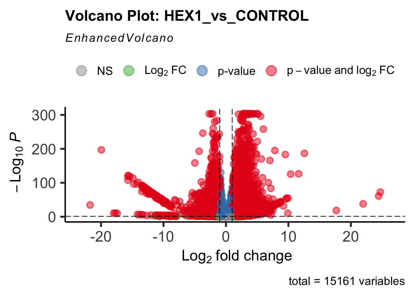
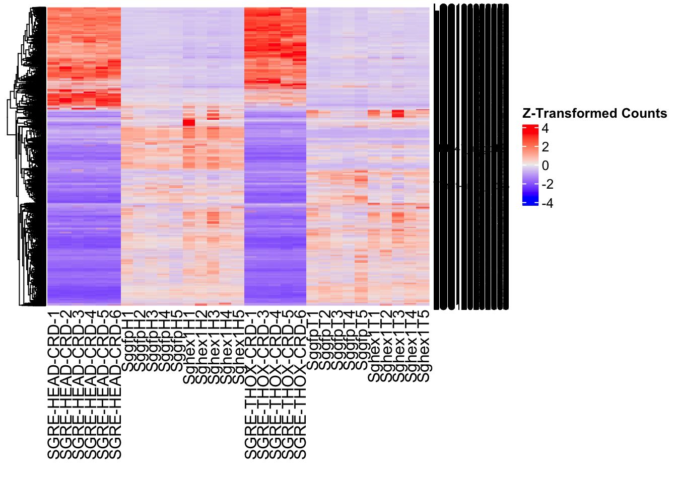
| Version | Author | Date |
|---|---|---|
| b540a1e | Maeva TECHER | 2025-02-27 |
hex2_plots$volcano; hex2_plots$heatmap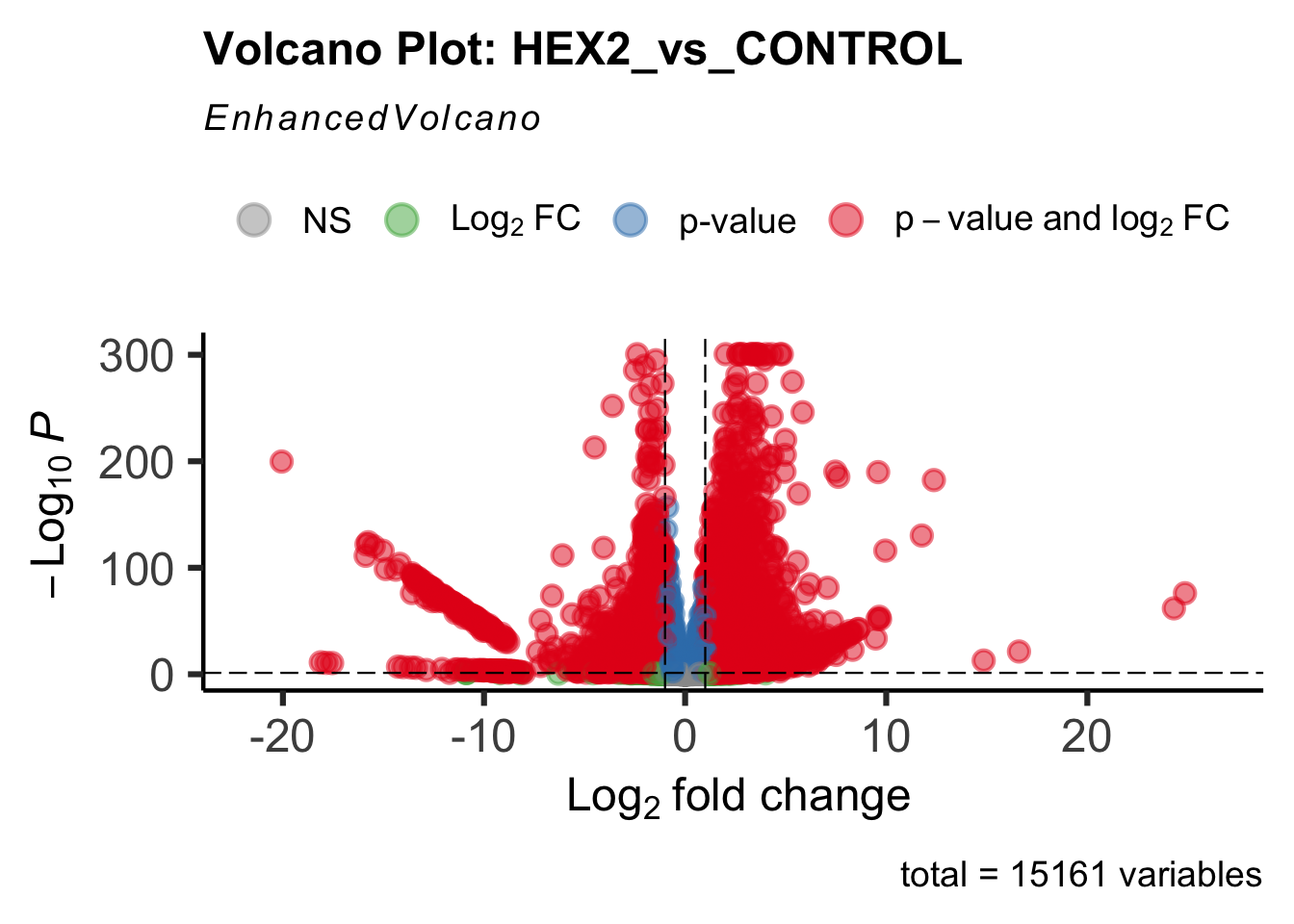
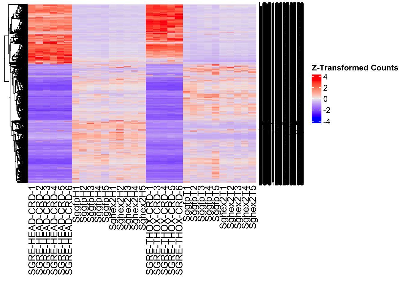
| Version | Author | Date |
|---|---|---|
| b540a1e | Maeva TECHER | 2025-02-27 |
jhmt_plots$volcano; jhmt_plots$heatmap
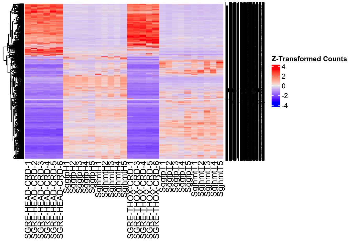
| Version | Author | Date |
|---|---|---|
| b540a1e | Maeva TECHER | 2025-02-27 |
miox_plots$volcano; miox_plots$heatmap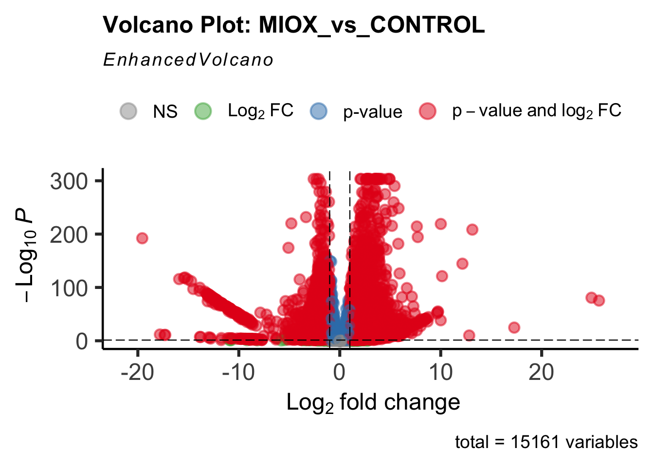
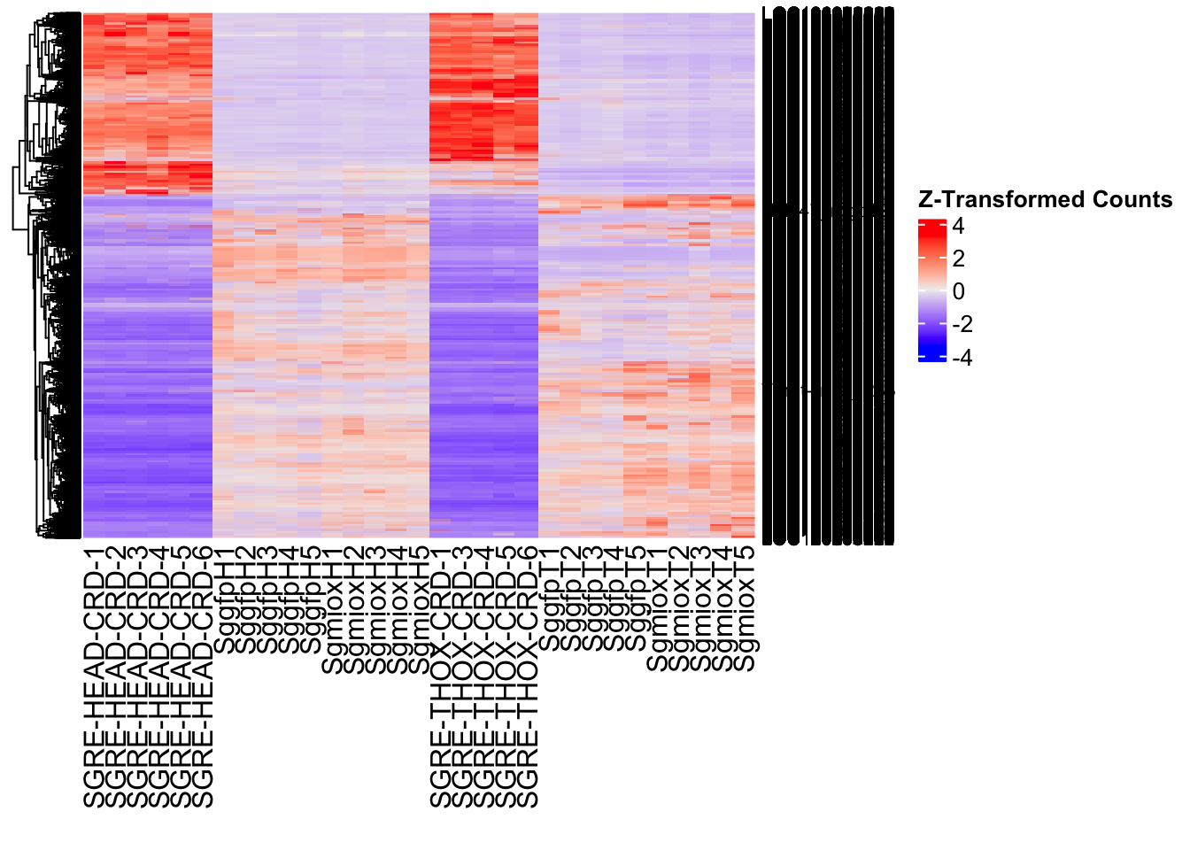
| Version | Author | Date |
|---|---|---|
| b540a1e | Maeva TECHER | 2025-02-27 |
unch_plots$volcano; unch_plots$heatmap
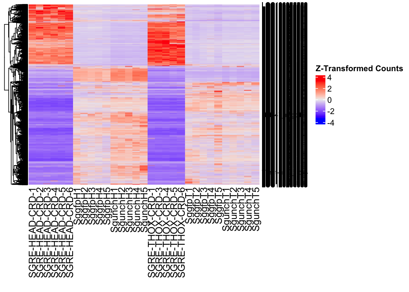
| Version | Author | Date |
|---|---|---|
| b540a1e | Maeva TECHER | 2025-02-27 |
gfp_plots$volcano; gfp_plots$heatmap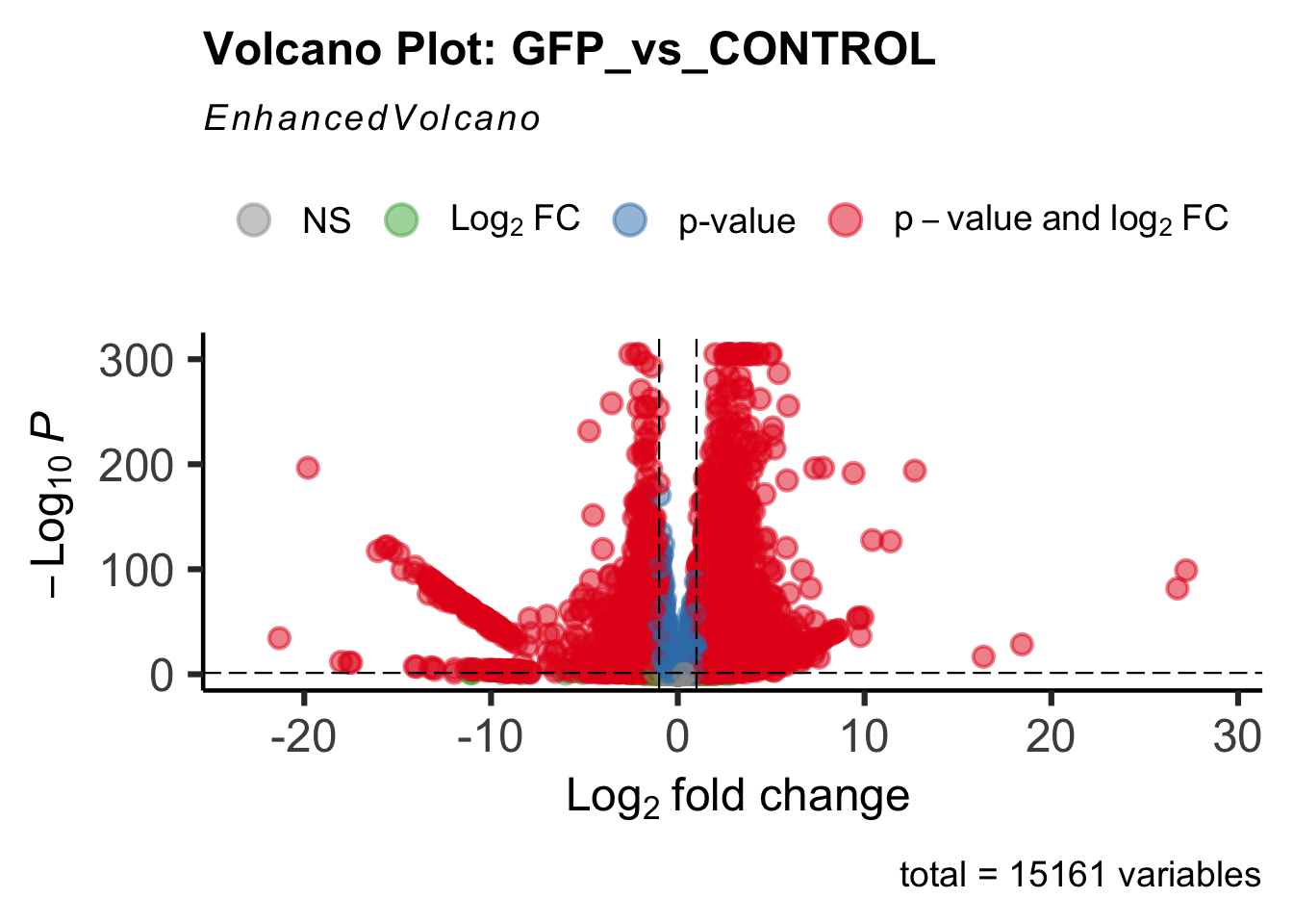
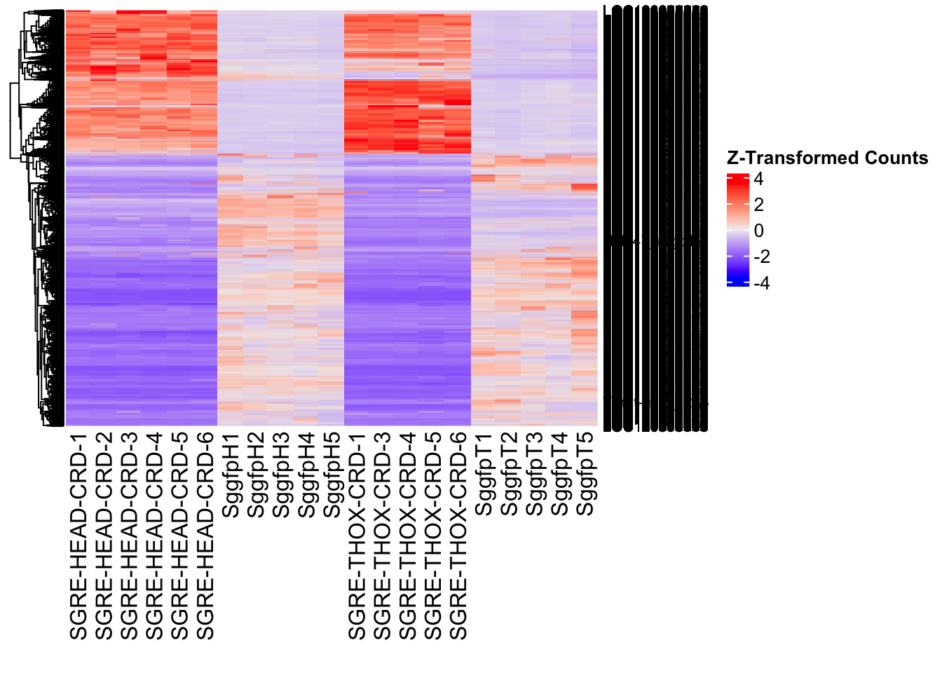
DEG tables
The following tables show the genes differentially expressed with at least an absolute log2fold change of > 1 considering all tissues together. Considering GFP as the reference state, upregulated genes in knockdown treatment in red and downregulated genes in knockdown treatment in blue. You can search for a gene of interest by writting a LOCID or description in the search bar or sort by column.
# Generate tables for each contrast
table_hex1 <- generate_deg_table(ddssva, "Gene_HEX1_vs_CONTROL", allspecies_df)
out of 15161 with nonzero total read count
adjusted p-value < 0.05
LFC > 0 (up) : 7668, 51%
LFC < 0 (down) : 4879, 32%
outliers [1] : 0, 0%
low counts [2] : 0, 0%
(mean count < 1)
[1] see 'cooksCutoff' argument of ?results
[2] see 'independentFiltering' argument of ?resultsTotal DEGs p-value < 0.05 and absolute logFoldChange > 1: 9098LFC > 1 (up) : 6002 (65.97%)LFC < -1 (down) : 3096 (34.03%)table_hex1$kable_tabletable_hex2 <- generate_deg_table(ddssva, "Gene_HEX2_vs_CONTROL", allspecies_df)
out of 15161 with nonzero total read count
adjusted p-value < 0.05
LFC > 0 (up) : 7470, 49%
LFC < 0 (down) : 4832, 32%
outliers [1] : 0, 0%
low counts [2] : 0, 0%
(mean count < 1)
[1] see 'cooksCutoff' argument of ?results
[2] see 'independentFiltering' argument of ?resultsTotal DEGs p-value < 0.05 and absolute logFoldChange > 1: 8642LFC > 1 (up) : 5728 (66.28%)LFC < -1 (down) : 2914 (33.72%)table_hex2$kable_tabletable_jhmt <- generate_deg_table(ddssva, "Gene_JHMT_vs_CONTROL", allspecies_df)
out of 15161 with nonzero total read count
adjusted p-value < 0.05
LFC > 0 (up) : 7722, 51%
LFC < 0 (down) : 4930, 33%
outliers [1] : 0, 0%
low counts [2] : 0, 0%
(mean count < 1)
[1] see 'cooksCutoff' argument of ?results
[2] see 'independentFiltering' argument of ?resultsTotal DEGs p-value < 0.05 and absolute logFoldChange > 1: 9086LFC > 1 (up) : 6006 (66.1%)LFC < -1 (down) : 3080 (33.9%)table_jhmt$kable_tabletable_miox <- generate_deg_table(ddssva, "Gene_MIOX_vs_CONTROL", allspecies_df)
out of 15161 with nonzero total read count
adjusted p-value < 0.05
LFC > 0 (up) : 7751, 51%
LFC < 0 (down) : 4955, 33%
outliers [1] : 0, 0%
low counts [2] : 0, 0%
(mean count < 1)
[1] see 'cooksCutoff' argument of ?results
[2] see 'independentFiltering' argument of ?resultsTotal DEGs p-value < 0.05 and absolute logFoldChange > 1: 9218LFC > 1 (up) : 6013 (65.23%)LFC < -1 (down) : 3205 (34.77%)table_miox$kable_tabletable_unch <- generate_deg_table(ddssva, "Gene_UNCH_vs_CONTROL", allspecies_df)
out of 15161 with nonzero total read count
adjusted p-value < 0.05
LFC > 0 (up) : 7724, 51%
LFC < 0 (down) : 4943, 33%
outliers [1] : 0, 0%
low counts [2] : 0, 0%
(mean count < 1)
[1] see 'cooksCutoff' argument of ?results
[2] see 'independentFiltering' argument of ?resultsTotal DEGs p-value < 0.05 and absolute logFoldChange > 1: 9155LFC > 1 (up) : 6002 (65.56%)LFC < -1 (down) : 3153 (34.44%)table_unch$kable_tabletable_gfp <- generate_deg_table(ddssva, "Gene_GFP_vs_CONTROL", allspecies_df)
out of 15161 with nonzero total read count
adjusted p-value < 0.05
LFC > 0 (up) : 7592, 50%
LFC < 0 (down) : 4963, 33%
outliers [1] : 0, 0%
low counts [2] : 0, 0%
(mean count < 1)
[1] see 'cooksCutoff' argument of ?results
[2] see 'independentFiltering' argument of ?resultsTotal DEGs p-value < 0.05 and absolute logFoldChange > 1: 8980LFC > 1 (up) : 5858 (65.23%)LFC < -1 (down) : 3122 (34.77%)table_gfp$kable_tableSummary and Overlap
# Summarize DEGs for all contrasts
deg_summary <- bind_rows(
summarize_deg_counts(table_hex1, "HEX1 vs CONTROL"),
summarize_deg_counts(table_hex2, "HEX2 vs CONTROL"),
summarize_deg_counts(table_jhmt, "JHMT vs CONTROL"),
summarize_deg_counts(table_miox, "MIOX vs CONTROL"),
summarize_deg_counts(table_unch, "UNCH vs CONTROL"),
summarize_deg_counts(table_gfp, "GFP vs CONTROL")
)
# Display table using kable with styling
deg_summary %>%
kable("html", escape = FALSE, col.names = gsub("_", " ", names(.))) %>%
kable_styling("striped", full_width = TRUE) %>%
column_spec(2, color = "red", bold = TRUE) %>% # Upregulated in red
column_spec(3, color = "blue", bold = TRUE) %>% # Downregulated in blue
add_header_above(c("Summary of DEGs" = 3)) %>%
row_spec(0, bold = TRUE)| Contrast | Upregulated | Downregulated |
|---|---|---|
| HEX1 vs CONTROL | 5980 | 3079 |
| HEX2 vs CONTROL | 5703 | 2895 |
| JHMT vs CONTROL | 5985 | 3064 |
| MIOX vs CONTROL | 5980 | 3187 |
| UNCH vs CONTROL | 5975 | 3137 |
| GFP vs CONTROL | 5823 | 3098 |
# Define the list of RNAi contrasts
contrast_list <- c("HEX1_vs_CONTROL", "HEX2_vs_CONTROL", "JHMT_vs_CONTROL",
"MIOX_vs_CONTROL", "UNCH_vs_CONTROL", "GFP_vs_CONTROL")
# Initialize empty lists for storing Head-specific DEGs for each contrast
venn_data_up <- list()
venn_data_down <- list()
venn_data_all <- list()
# Function to load Head-specific DEGs for a given set of contrasts
load_deg_contrasts_head <- function(contrast_list) {
degs_up <- list()
degs_down <- list()
degs_all <- list()
for (contrast in contrast_list) {
deg_file <- file.path(workDir, "DEG_results/RNAi/All_control_no_rRNA/", contrast, paste0("DEG_sigresults_", contrast, ".csv"))
if (!file.exists(deg_file)) {
message(paste("File missing for contrast:", contrast))
next # Skip if the file doesn't exist
}
deg_data <- read.csv(deg_file, stringsAsFactors = FALSE)
# Convert row names to a column if necessary
if ("X" %in% colnames(deg_data)) {
colnames(deg_data)[colnames(deg_data) == "X"] <- "GeneID"
}
# Check if data is empty
if (nrow(deg_data) == 0) {
message(paste("No data for contrast:", contrast))
next
}
# Select significant DEGs (Up, Down, All)
degs_up[[contrast]] <- deg_data %>%
filter(padj < 0.05 & log2FoldChange >= 1) %>%
pull(GeneID) # Extract GeneID column
degs_down[[contrast]] <- deg_data %>%
filter(padj < 0.05 & log2FoldChange <= -1) %>%
pull(GeneID) # Extract GeneID column
degs_all[[contrast]] <- deg_data %>%
filter(padj < 0.05 & abs(log2FoldChange) >= 1) %>%
pull(GeneID) # Extract GeneID column
}
return(list(up = degs_up, down = degs_down, all = degs_all))
}
# Load DEG data for the defined contrasts (Head tissue only)
venn_data_contrasts <- load_deg_contrasts_head(contrast_list)
# Prepare the data for the Venn diagrams
venn_data_up <- venn_data_contrasts$up
venn_data_down <- venn_data_contrasts$down
venn_data_all <- venn_data_contrasts$all
# Display the Venn diagram and datatable for **Head Upregulated DEGs** across contrasts
display_ggvenn_plot(venn_data_up, "Venn Diagram of Head and Thorax Upregulated DEGs - RNAi Contrasts")
# Display the Venn diagram and datatable for **Head Downregulated DEGs** across contrasts
display_ggvenn_plot(venn_data_down, "Venn Diagram of Head and Thorax Downregulated DEGs - RNAi Contrasts")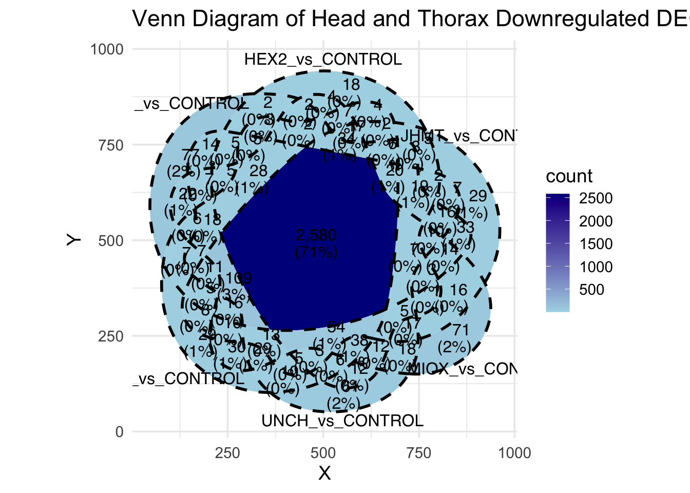
# Display the Venn diagram and datatable for **All Significant DEGs in Head Tissue**
display_ggvenn_plot(venn_data_all, "Venn Diagram of All Significant DEGs in All Tissue - RNAi Contrasts")
# Run the UpSet plot for Head Upregulated DEGs
display_upset_plot(venn_data_up, "UpSet Plot of Head and Thorax Upregulated DEGs - RNAi Contrasts")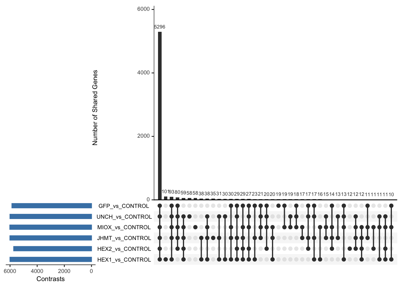
# Run the UpSet plot for Head Downregulated DEGs
display_upset_plot(venn_data_down, "UpSet Plot of Head and Thorax Downregulated DEGs - RNAi Contrasts")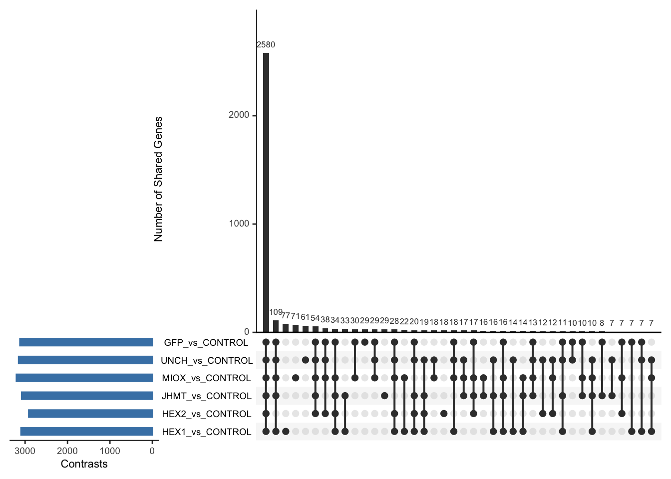
# Run the UpSet plot for Head Upregulated DEGs
display_upset_plot(venn_data_all, "UpSet Plot of All Significant DEGs in All Tissue - RNAi Contrasts")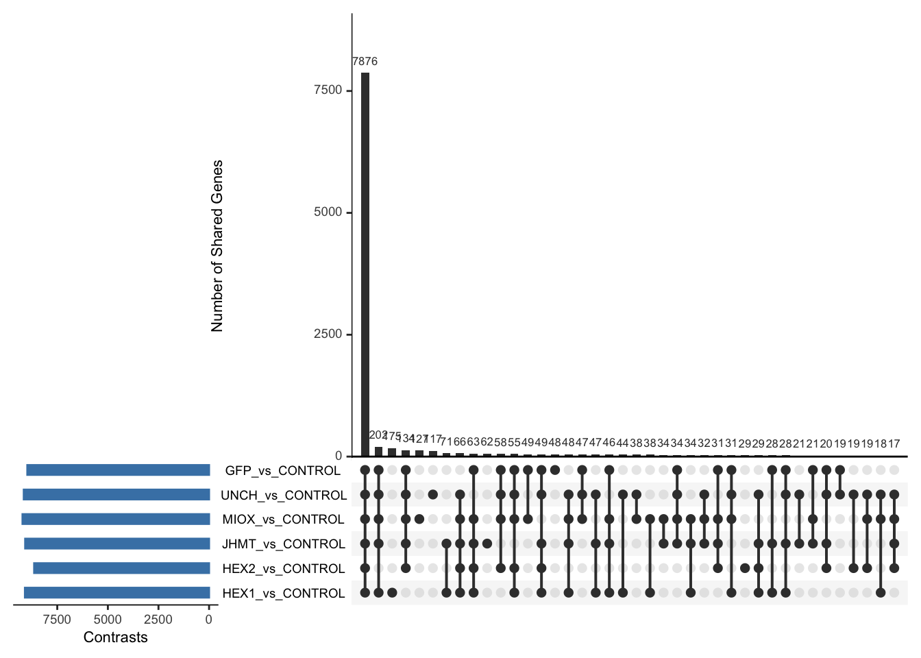
Head tissue
saveDir <- paste0(workDir,"/DEG_results/RNAi/Head_control_no_rRNA")
dir.create(saveDir)
### Prepare Sample CSV file #####
samples <- read.delim(file.path(workDir, "list/RNAi/Head_RNAi_noninjectedsample_list.csv"), sep = ",", row.names = 1, header = TRUE)
files <- file.path(workDir, "readcounts/RNAi/", samples$Tissue, samples$Filename)
names(files) <- row.names(samples)
if (all(file.exists(files))) {
message("All the files exist!")
} else {
warning("Some files are missing!")
}All the files exist!### **Standardized Count Matrix Creation**
# Extract all gene lists first
gene_lists <- map(files, function(sample) {
fread(sample, sep = "\t", header = FALSE)[, 1] # Extract Gene IDs (column 1)
})
# Get a unique set of all gene IDs across all samples
all_genes <- unique(unlist(gene_lists))
# Create a named list to store count data with standardized rows
cts_list <- map(files, function(sample) {
data_count <- fread(sample, sep = "\t", header = FALSE)
col_name <- gsub("_counts.txt", "", basename(sample)) # Clean sample name
# Convert to data frame with correct column names
data_count <- setNames(data.frame(data_count[, 1:2]), c("GeneID", col_name))
# Ensure all gene IDs are present (fill missing values with 0)
data_count <- full_join(data.frame(GeneID = all_genes), data_count, by = "GeneID") %>%
mutate(across(where(is.numeric), ~ replace_na(., 0))) # Fill NA with 0
return(data_count)
})
# Merge all samples based on GeneID
cts <- reduce(cts_list, full_join, by = "GeneID")
# Convert to matrix for DESeq2
cts_matrix <- as.matrix(cts[, -1]) # Remove GeneID column for count matrix
rownames(cts_matrix) <- cts$GeneID # Set GeneID as rownames
rm(cts_list) # Free memoryWhile for bulk RNAseq on head and thorax for all species, the DEGs model was made between isolated and crowded individuals (with isolated as the reference state), here, the DEG analysis will be carried between GFP knock-down nymphs (as reference state) vs Hexamerins / Juvenile Hormones / Inositol / Uncharacterized proteins.
### Build DESeq2 Object
dds <- DESeqDataSetFromMatrix(countData = cts_matrix,
colData = samples,
design = ~ Gene)
dds$Gene <- relevel(dds$Gene, ref = "CONTROL")
smallestGroupSize <- 5
keep <- rowSums(counts(dds) >= 10) >= smallestGroupSize
dds <- dds[keep,]
loci_to_exclude <- readLines(file.path(workDir, "list/excluded_loci/gregaria_rrna_list.txt"))
dds <- dds[!(rownames(dds) %in% loci_to_exclude), ]
dds <- DESeq(dds)Normalization and PCA
# Plot PCA and investigate quality metrics
vsd <- vst(dds, blind = TRUE)
# Perform PCA
pca_data <- plotPCA(vsd, intgroup = c("Tissue", "Gene"), returnData = TRUE)
# Define colors for genes (slightly transparent) and shapes for tissues
gene_colors <- scale_color_manual(values = alpha(brewer.pal(n = length(unique(pca_data$Gene)), name = "Set1"), 0.8)) # Points are transparent
tissue_shapes <- scale_shape_manual(values = seq(15, 15 + length(unique(pca_data$Tissue))))
# **PCA without labels**
p_pca_nolabel <- ggplot(pca_data, aes(x = PC1, y = PC2, color = Gene, shape = Tissue)) +
geom_point(size = 4) +
gene_colors +
tissue_shapes +
theme_bw() +
theme(legend.title = element_blank(),
legend.text = element_text(face = "bold", size = 14),
axis.text = element_text(size = 12),
axis.title = element_text(size = 14)) +
ggtitle("PCA of All Tissues (No Labels)", subtitle = "Tissues differentiated by shape, Genes by color")
# Save PCA without labels
ggsave(paste0(saveDir, "/PCA_Tissue_Gene_NoLabel.png"), plot = p_pca_nolabel, width = 10, height = 10, dpi = 600, device = "png")
# **PCA with labels**
p_pca_label <- ggplot(pca_data, aes(x = PC1, y = PC2, color = Gene, shape = Tissue)) +
geom_point(size = 4) +
geom_text_repel(aes(label = name), size = 4, color = "black", max.overlaps = 20) + # Labels are fully visible
gene_colors +
tissue_shapes +
theme_bw() +
theme(legend.title = element_blank(),
legend.text = element_text(face = "bold", size = 14),
axis.text = element_text(size = 12),
axis.title = element_text(size = 14)) +
ggtitle("PCA of All Tissues (With Labels)", subtitle = "Tissues differentiated by shape, Genes by color")
# Save PCA with labels
ggsave(paste0(saveDir, "/PCA_Tissue_Gene_Label.png"), plot = p_pca_label, width = 10, height = 10, dpi = 600, device = "png")
# **Return plots for knitr/RMarkdown**
list(NoLabel = p_pca_nolabel, WithLabel = p_pca_label)$NoLabel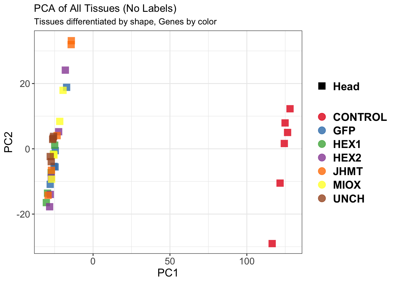
| Version | Author | Date |
|---|---|---|
| b540a1e | Maeva TECHER | 2025-02-27 |
$WithLabel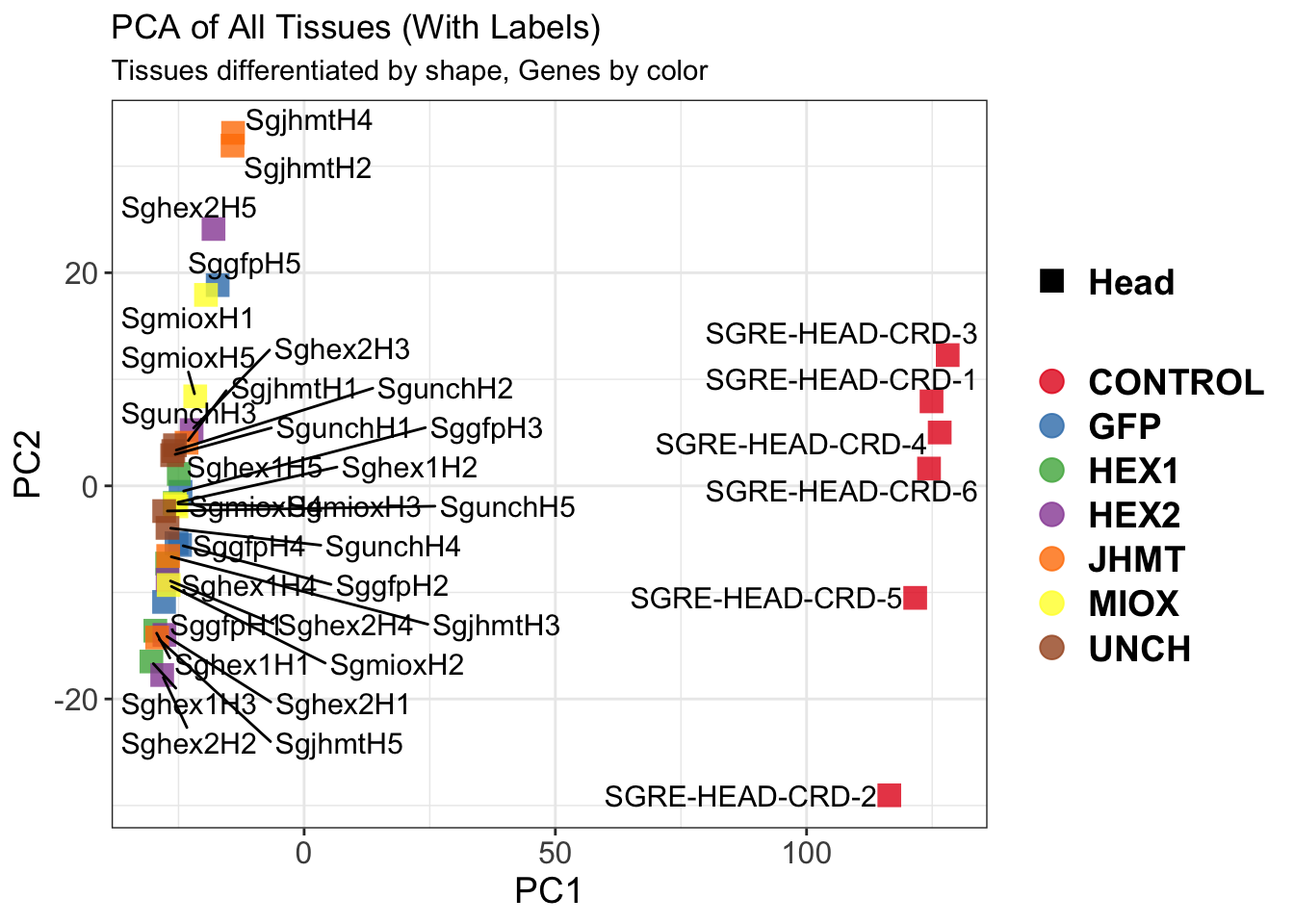
| Version | Author | Date |
|---|---|---|
| b540a1e | Maeva TECHER | 2025-02-27 |
The PCA plot shows clear distinction between tissue types, while gene silencing has a large variation within each tissue, and presents no distinct clear groupings for a single gene.
SVA
### SVA analysis to control for technical variation
dat <- counts(dds, normalized = TRUE)
idx <- rowMeans(dat) > 1
dat <- dat[idx, ]
mod <- model.matrix(~ Gene, colData(dds))
mod0 <- model.matrix(~ 1, colData(dds))
svseq <- svaseq(dat, mod, mod0)Number of significant surrogate variables is: 7
Iteration (out of 5 ):1 2 3 4 5 sva_plots <- create_sva_plots(svseq, dds, saveDir, intgroup = c("Tissue", "Gene"), max_sv = 7)
# Show stripcharts in the report
sva_plots$Stripcharts[[1]] # Show first stripchart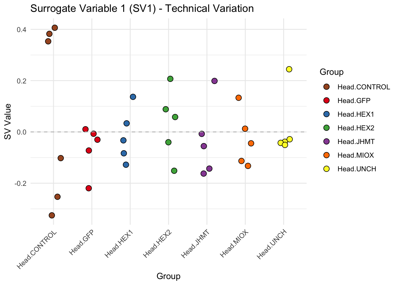
| Version | Author | Date |
|---|---|---|
| b540a1e | Maeva TECHER | 2025-02-27 |
sva_plots$Stripcharts[[2]] # Show second stripchart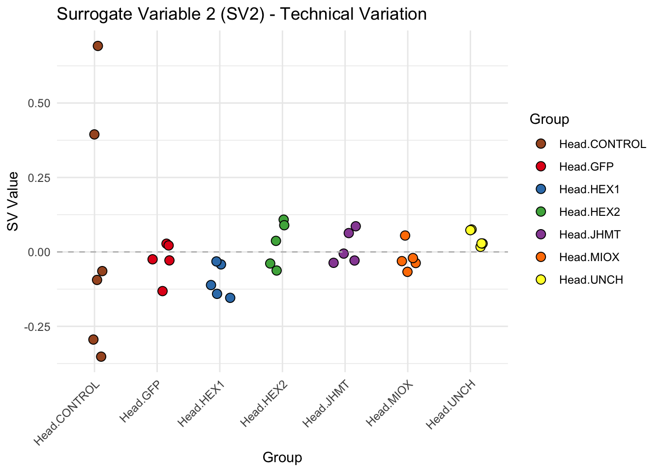
| Version | Author | Date |
|---|---|---|
| b540a1e | Maeva TECHER | 2025-02-27 |
sva_plots$Stripcharts[[3]] # Show third stripchart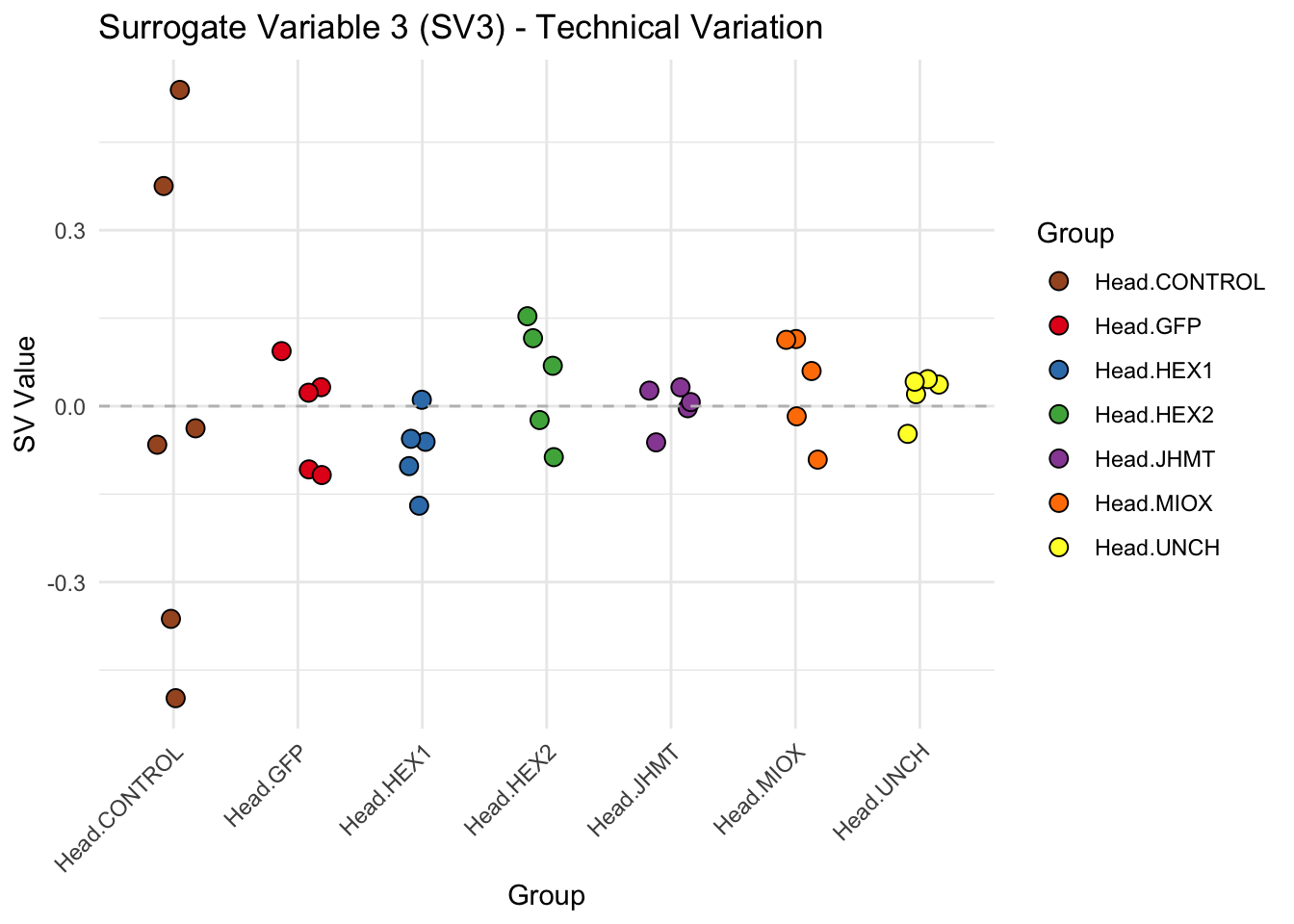
| Version | Author | Date |
|---|---|---|
| b540a1e | Maeva TECHER | 2025-02-27 |
sva_plots$Stripcharts[[4]] 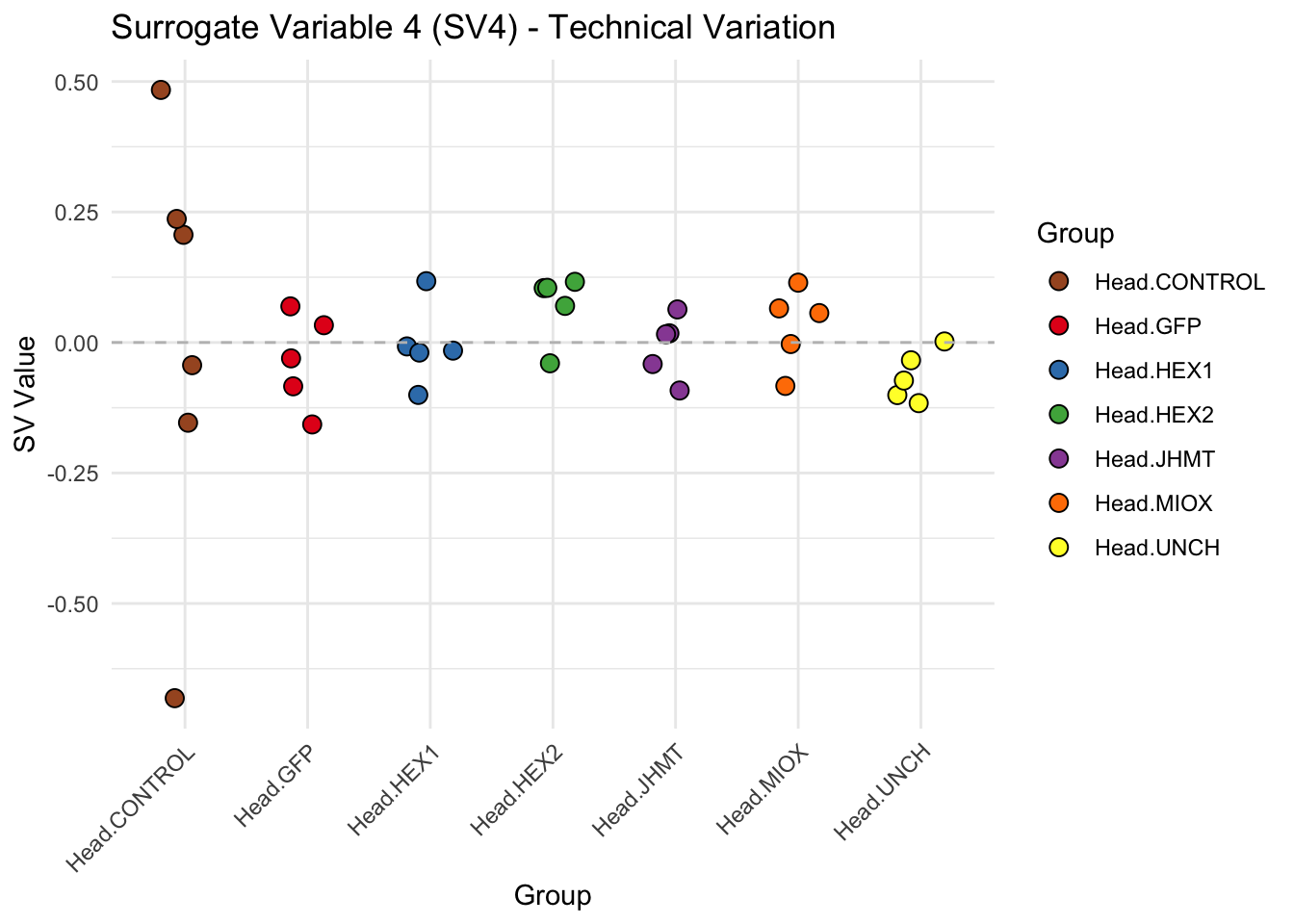
| Version | Author | Date |
|---|---|---|
| b540a1e | Maeva TECHER | 2025-02-27 |
sva_plots$Stripcharts[[5]] # Show second stripchart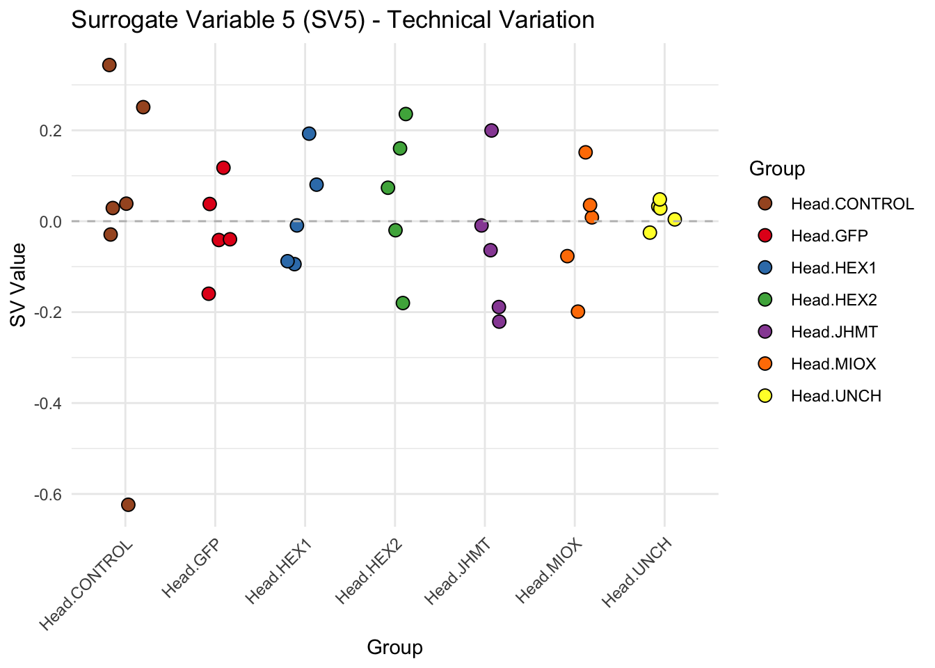
| Version | Author | Date |
|---|---|---|
| b540a1e | Maeva TECHER | 2025-02-27 |
sva_plots$Stripcharts[[6]] # Show third stripchart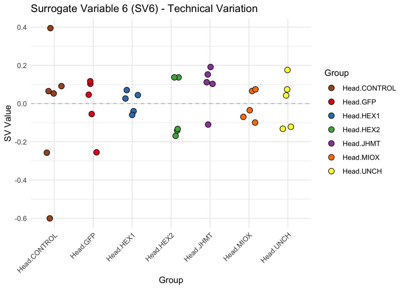
| Version | Author | Date |
|---|---|---|
| b540a1e | Maeva TECHER | 2025-02-27 |
sva_plots$Stripcharts[[7]] 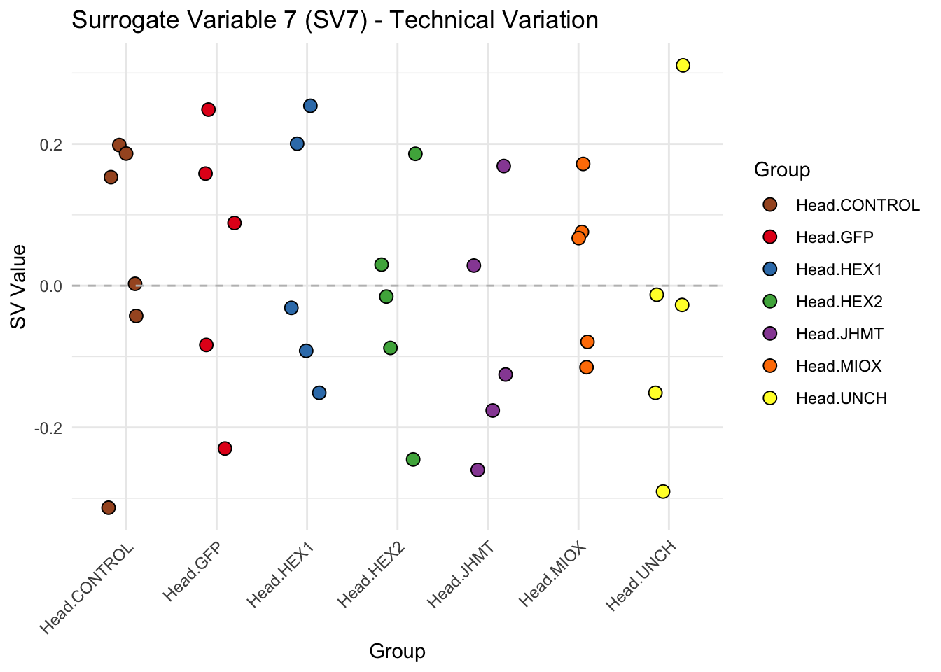
| Version | Author | Date |
|---|---|---|
| b540a1e | Maeva TECHER | 2025-02-27 |
# Show scatter plots in the report
sva_plots$ScatterPlots[["1_2"]] # Show SV1 vs SV2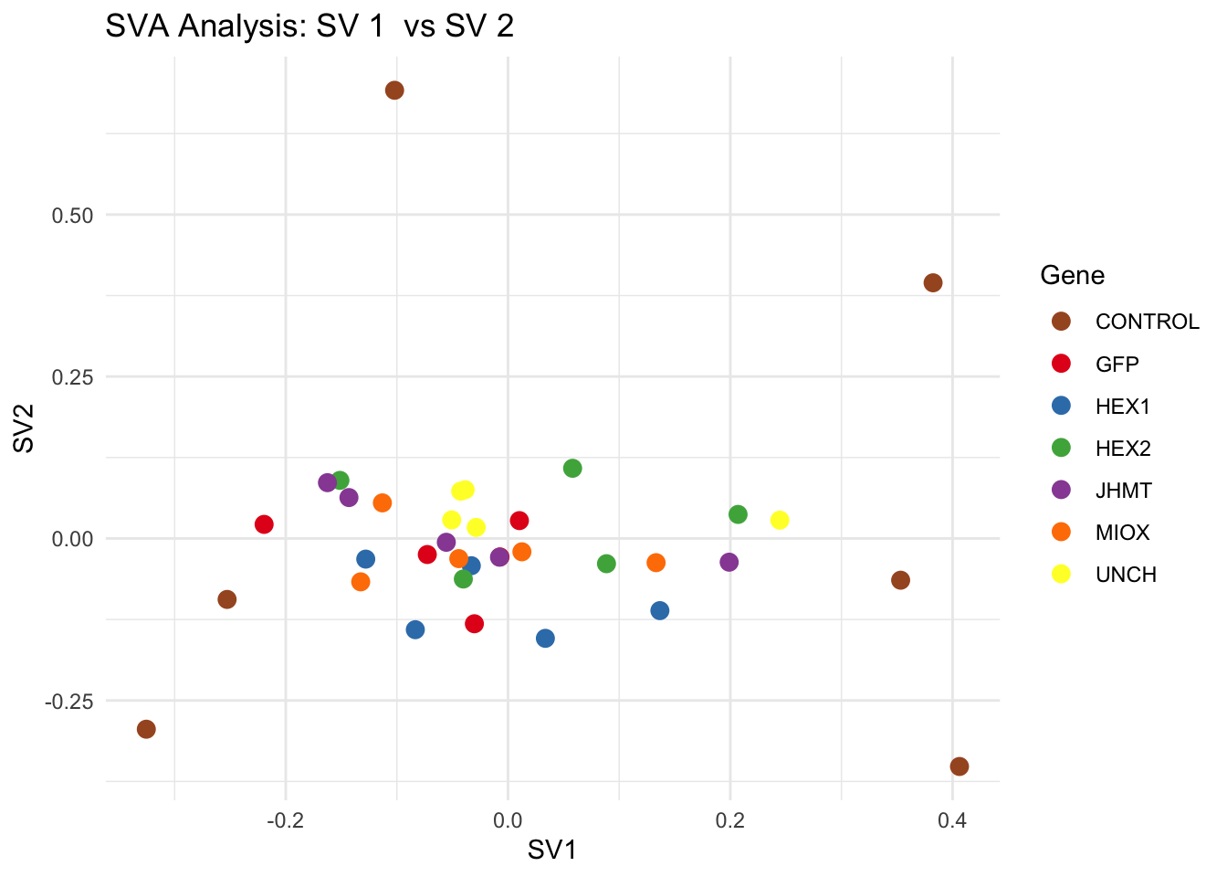
| Version | Author | Date |
|---|---|---|
| b540a1e | Maeva TECHER | 2025-02-27 |
sva_plots$ScatterPlots[["1_3"]] # Show SV1 vs SV3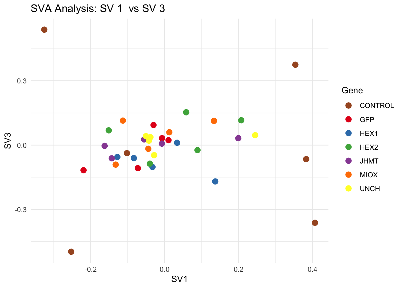
| Version | Author | Date |
|---|---|---|
| b540a1e | Maeva TECHER | 2025-02-27 |
sva_plots$ScatterPlots[["2_3"]] # Show SV2 vs SV3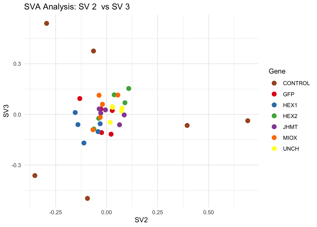
| Version | Author | Date |
|---|---|---|
| b540a1e | Maeva TECHER | 2025-02-27 |
SV1 is clearly showing an effect of tissue. We rerun the
DESeq2 model but this time including the surrogate variable
SV2 and SV3 as a covariates only, as we know that the modeled variation
is more likely explained by tissue and gene variation rather than batch
effects.
ddssva <- dds
ddssva$SV1 <- svseq$sv[,1]
ddssva$SV2 <- svseq$sv[,2]
ddssva$SV3 <- svseq$sv[,3]
ddssva$SV4 <- svseq$sv[,4]
ddssva$SV5 <- svseq$sv[,5]
ddssva$SV6 <- svseq$sv[,6]
ddssva$SV7 <- svseq$sv[,7]
design(ddssva) <- ~ SV1 + SV2 + SV3 + SV4 + SV5 + SV6 + SV7 + Gene
ddssva$Gene <- relevel(ddssva$Gene, ref = "CONTROL")
smallestGroupSize <- 5
keep <- rowSums(counts(ddssva) >= 10) >= smallestGroupSize
ddssva <- ddssva[keep,]
ddssva <- DESeq(ddssva)
ddssva <- ddssva[which(mcols(ddssva)$betaConv),] # remove non converging rows
### Extract results
message("Available contrasts are: ", paste(resultsNames(ddssva), collapse = ", "))
hex1 <- results(ddssva, contrast = c("Gene", "HEX1", "CONTROL"), alpha = 0.05)
hex2 <- results(ddssva, contrast = c("Gene", "HEX2", "CONTROL"), alpha = 0.05)
jhmt <- results(ddssva, contrast = c("Gene", "JHMT", "CONTROL"), alpha = 0.05)
miox <- results(ddssva, contrast = c("Gene", "MIOX", "CONTROL"), alpha = 0.05)
unch <- results(ddssva, contrast = c("Gene", "UNCH", "CONTROL"), alpha = 0.05)
gfp <- results(ddssva, contrast = c("Gene", "GFP", "CONTROL"), alpha = 0.05)Volcano plots and Heatmaps
# Define contrast_sets
hex1_samples <- c("SGRE-HEAD-CRD-1","SGRE-HEAD-CRD-2","SGRE-HEAD-CRD-3","SGRE-HEAD-CRD-4","SGRE-HEAD-CRD-5",
"SGRE-HEAD-CRD-6","SggfpH1","SggfpH2","SggfpH3","SggfpH4","SggfpH5",
"Sghex1H1","Sghex1H2","Sghex1H3","Sghex1H4","Sghex1H5")
hex2_samples <- c("SGRE-HEAD-CRD-1","SGRE-HEAD-CRD-2","SGRE-HEAD-CRD-3","SGRE-HEAD-CRD-4","SGRE-HEAD-CRD-5",
"SGRE-HEAD-CRD-6","SggfpH1","SggfpH2","SggfpH3","SggfpH4","SggfpH5",
"Sghex2H1","Sghex2H2","Sghex2H3","Sghex2H4","Sghex2H5")
jhmt_samples <- c("SGRE-HEAD-CRD-1","SGRE-HEAD-CRD-2","SGRE-HEAD-CRD-3","SGRE-HEAD-CRD-4","SGRE-HEAD-CRD-5",
"SGRE-HEAD-CRD-6","SggfpH1","SggfpH2","SggfpH3","SggfpH4","SggfpH5",
"SgjhmtH1","SgjhmtH2","SgjhmtH3","SgjhmtH4","SgjhmtH5")
miox_samples <- c("SGRE-HEAD-CRD-1","SGRE-HEAD-CRD-2","SGRE-HEAD-CRD-3","SGRE-HEAD-CRD-4","SGRE-HEAD-CRD-5",
"SGRE-HEAD-CRD-6","SggfpH1","SggfpH2","SggfpH3","SggfpH4","SggfpH5",
"SgmioxH1","SgmioxH2","SgmioxH3","SgmioxH4","SgmioxH5")
unch_samples <- c("SGRE-HEAD-CRD-1","SGRE-HEAD-CRD-2","SGRE-HEAD-CRD-3","SGRE-HEAD-CRD-4","SGRE-HEAD-CRD-5",
"SGRE-HEAD-CRD-6","SggfpH1","SggfpH2","SggfpH3","SggfpH4","SggfpH5",
"SgunchH1","SgunchH2","SgunchH3","SgunchH4","SgunchH5")
gfp_samples <- c("SGRE-HEAD-CRD-1","SGRE-HEAD-CRD-2","SGRE-HEAD-CRD-3","SGRE-HEAD-CRD-4","SGRE-HEAD-CRD-5",
"SGRE-HEAD-CRD-6","SggfpH1","SggfpH2","SggfpH3","SggfpH4","SggfpH5")
# Run full analysis
hex1_plots <- visualize_data_nopng(hex1, "HEX1_vs_CONTROL", hex1_samples)
hex2_plots <- visualize_data_nopng(hex2, "HEX2_vs_CONTROL", hex2_samples)
jhmt_plots <- visualize_data_nopng(jhmt, "JHMT_vs_CONTROL", jhmt_samples)
miox_plots <- visualize_data_nopng(miox, "MIOX_vs_CONTROL", miox_samples)
unch_plots <- visualize_data_nopng(unch, "UNCH_vs_CONTROL", unch_samples)
gfp_plots <- visualize_data_nopng(gfp, "GFP_vs_CONTROL", gfp_samples)
hex1_plots$volcano; hex1_plots$heatmap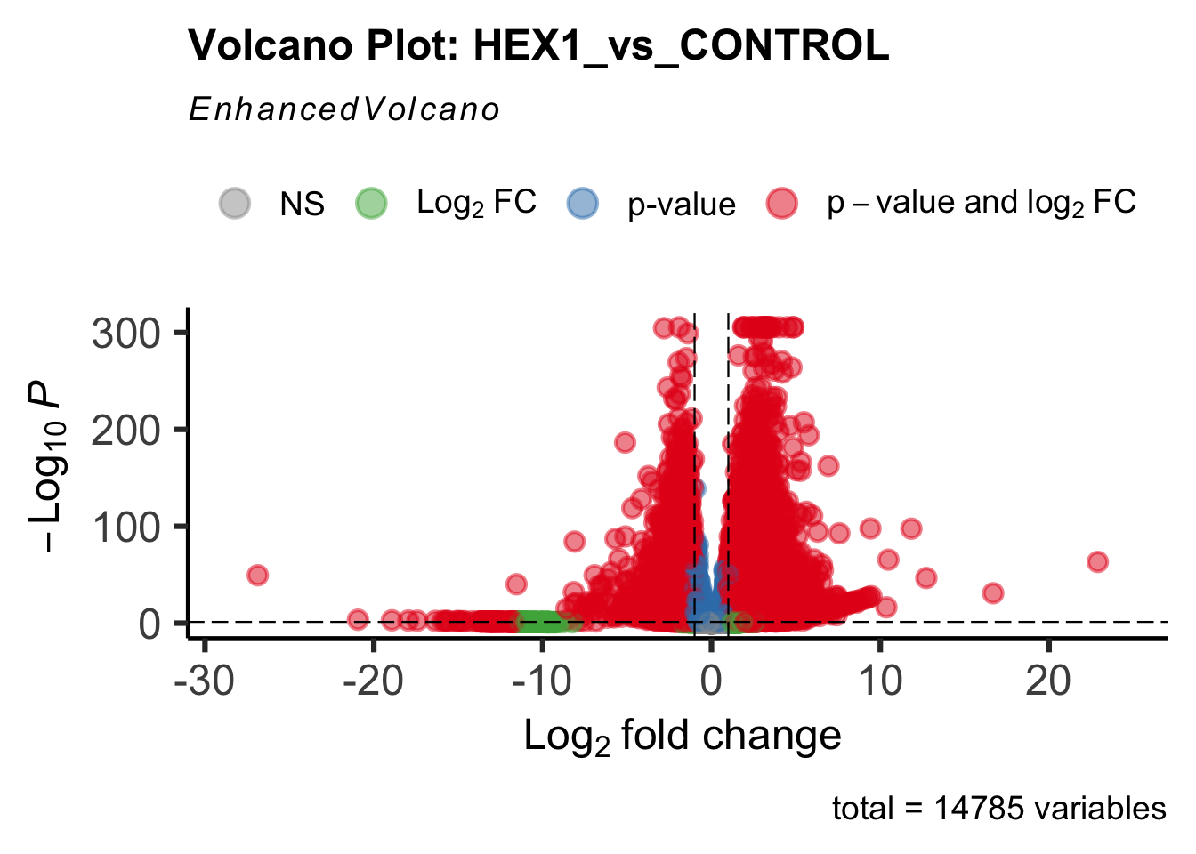
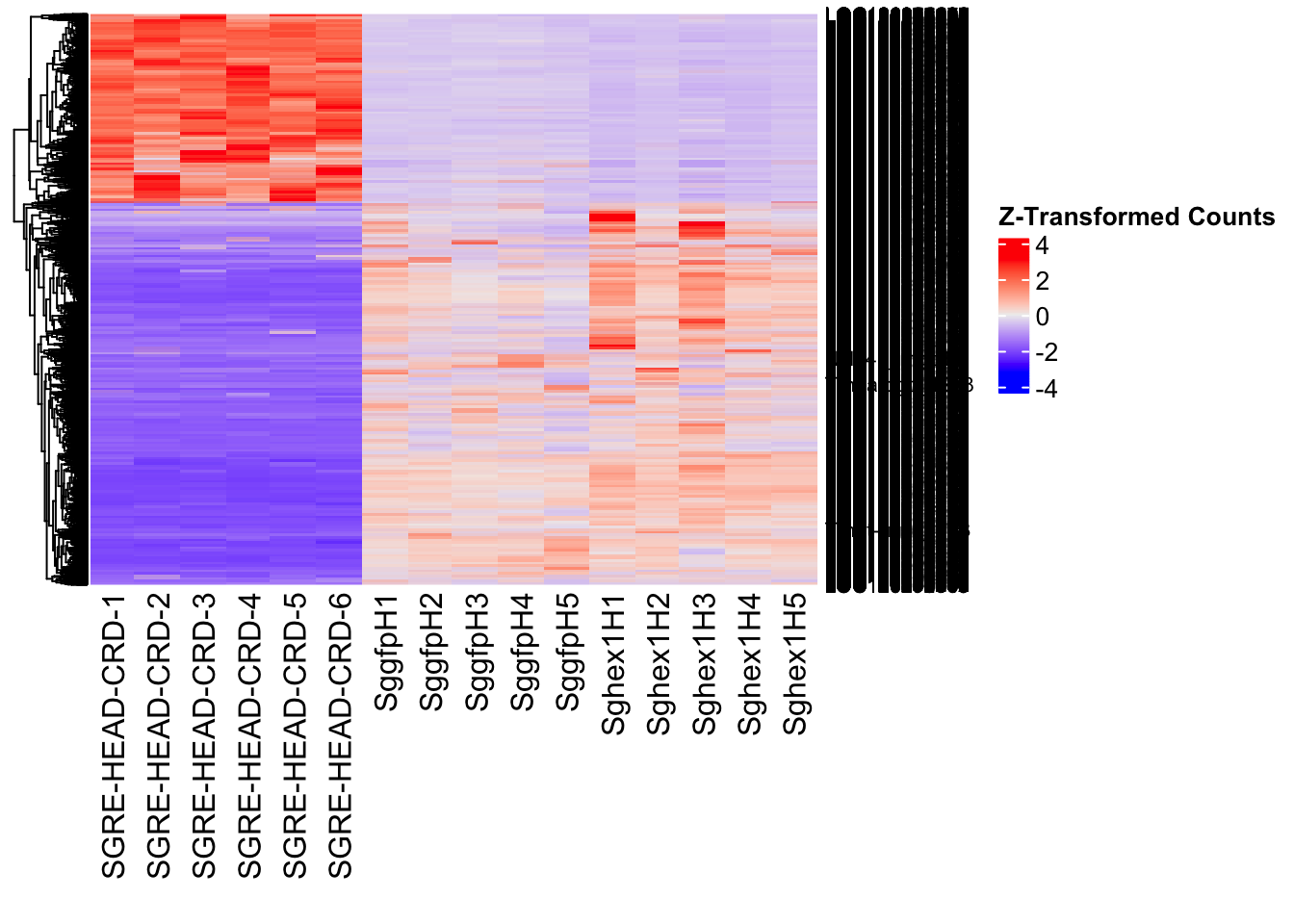
| Version | Author | Date |
|---|---|---|
| b540a1e | Maeva TECHER | 2025-02-27 |
hex2_plots$volcano; hex2_plots$heatmap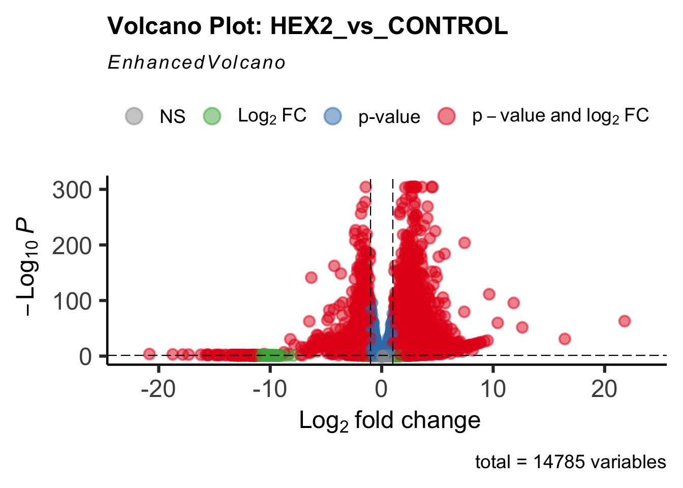
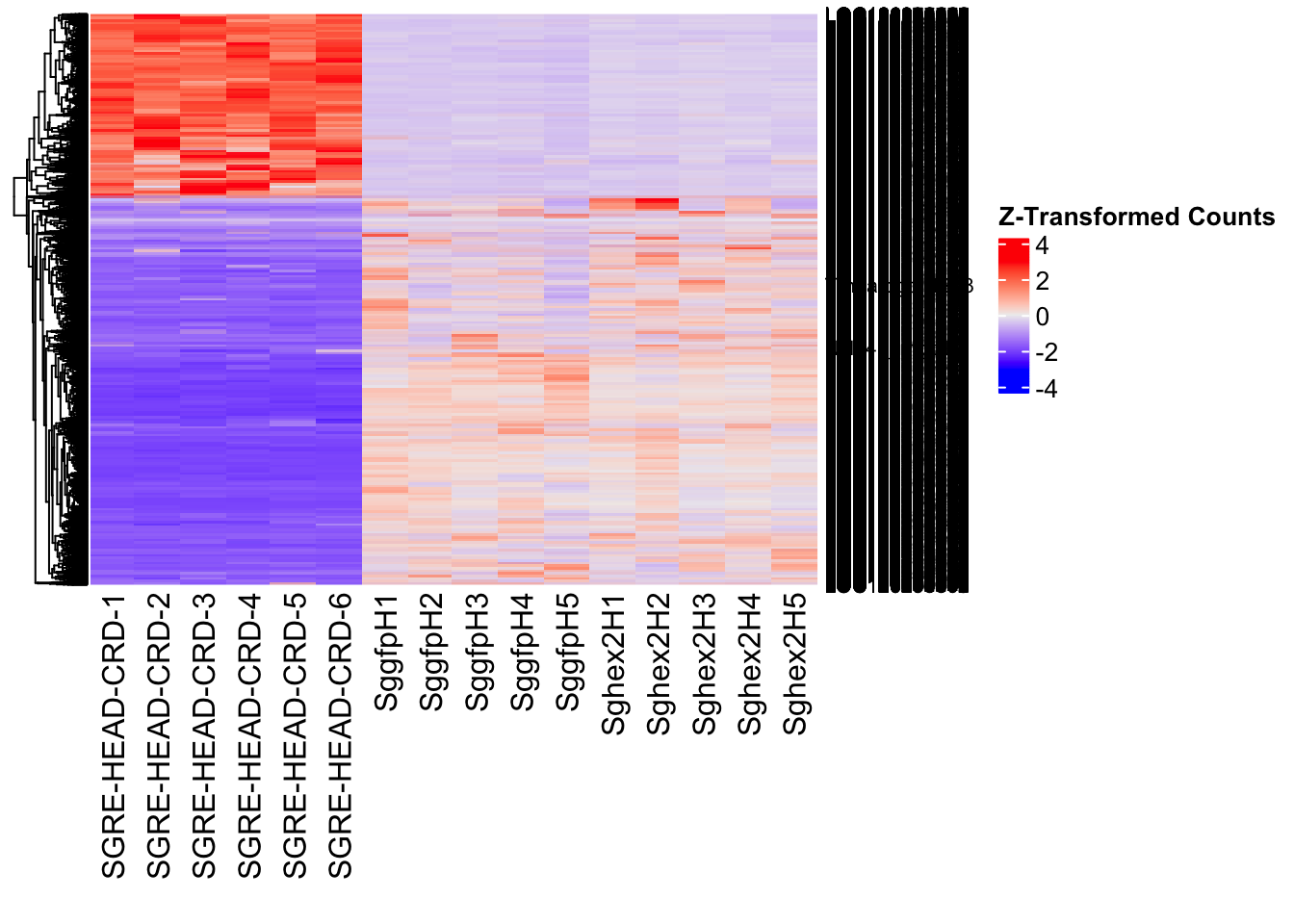
| Version | Author | Date |
|---|---|---|
| b540a1e | Maeva TECHER | 2025-02-27 |
jhmt_plots$volcano; jhmt_plots$heatmap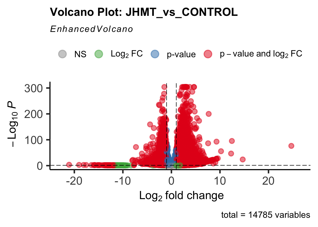
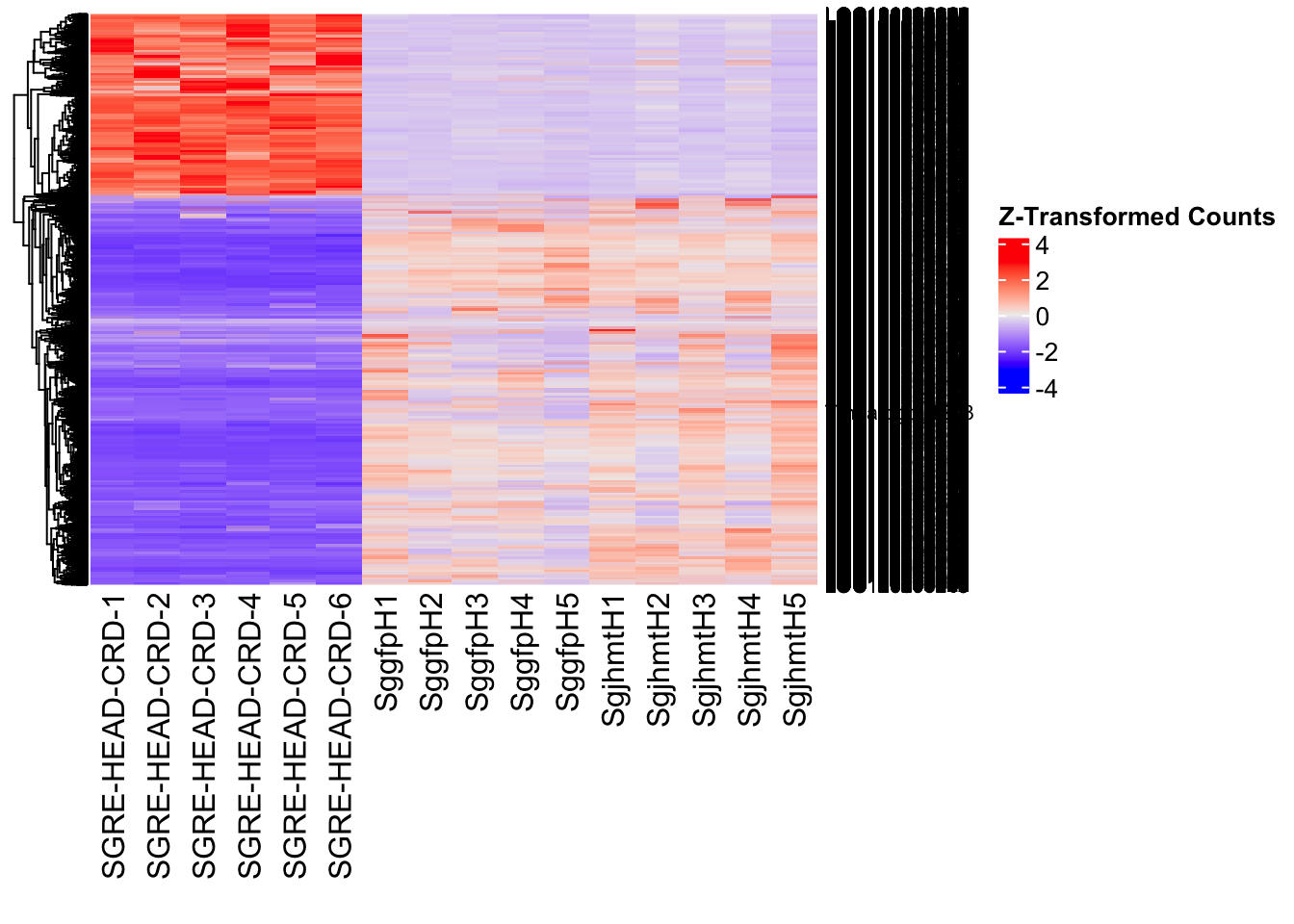
| Version | Author | Date |
|---|---|---|
| b540a1e | Maeva TECHER | 2025-02-27 |
miox_plots$volcano; miox_plots$heatmap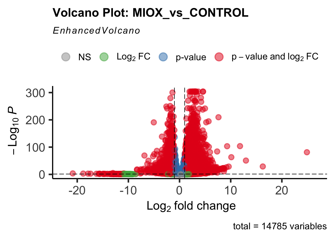
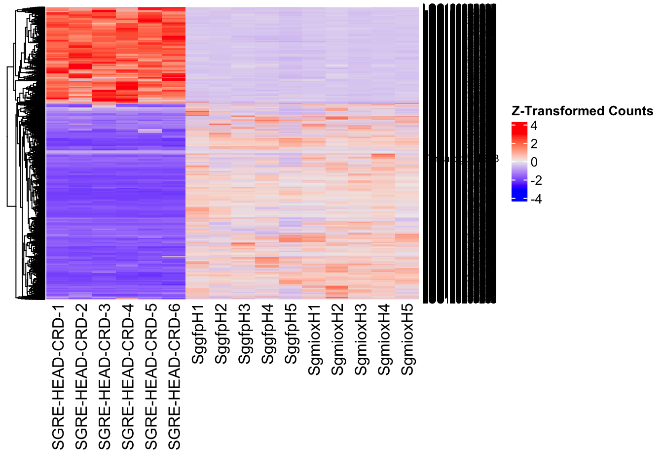
| Version | Author | Date |
|---|---|---|
| b540a1e | Maeva TECHER | 2025-02-27 |
unch_plots$volcano; unch_plots$heatmap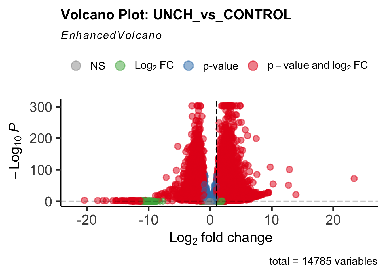
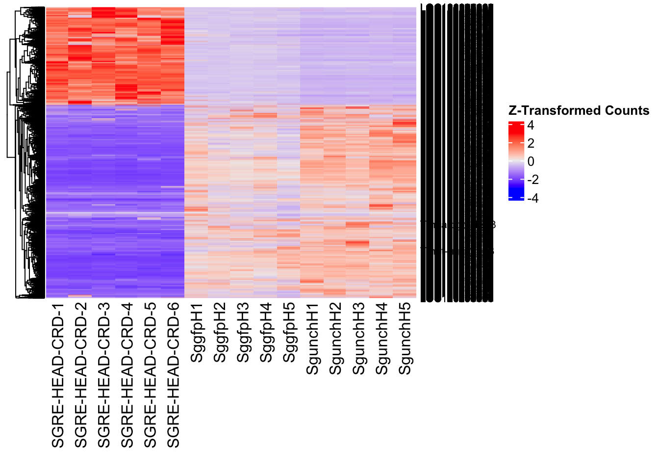
gfp_plots$volcano; gfp_plots$heatmap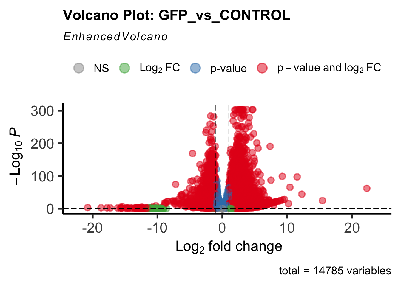
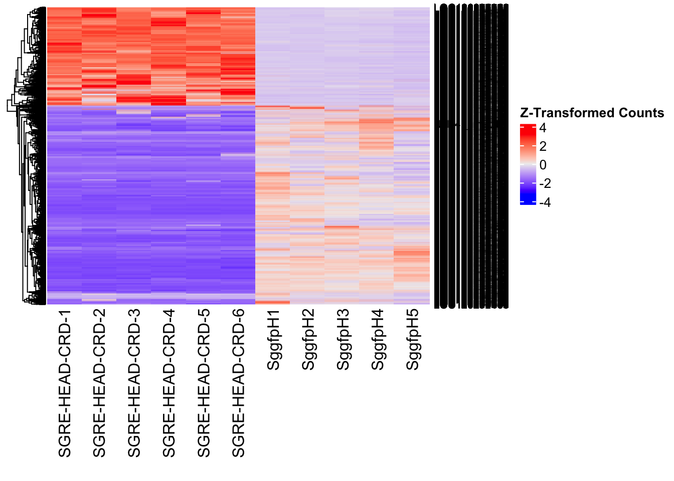
DEG tables
The following tables show the genes differentially expressed with at least an absolute log2fold change of > 1 considering Head tissues only. Considering GFP as the reference state, upregulated genes in knockdown treatment in red and downregulated genes in knockdown treatment in blue. You can search for a gene of interest by writting a LOCID or description in the search bar or sort by column.
# Generate tables for each contrast
table_hex1 <- generate_deg_table(ddssva, "Gene_HEX1_vs_CONTROL", allspecies_df)
out of 14785 with nonzero total read count
adjusted p-value < 0.05
LFC > 0 (up) : 7507, 51%
LFC < 0 (down) : 4600, 31%
outliers [1] : 0, 0%
low counts [2] : 0, 0%
(mean count < 2)
[1] see 'cooksCutoff' argument of ?results
[2] see 'independentFiltering' argument of ?resultsTotal DEGs p-value < 0.05 and absolute logFoldChange > 1: 8836LFC > 1 (up) : 5921 (67.01%)LFC < -1 (down) : 2915 (32.99%)table_hex1$kable_tabletable_hex2 <- generate_deg_table(ddssva, "Gene_HEX2_vs_CONTROL", allspecies_df)
out of 14785 with nonzero total read count
adjusted p-value < 0.05
LFC > 0 (up) : 7177, 49%
LFC < 0 (down) : 4533, 31%
outliers [1] : 0, 0%
low counts [2] : 0, 0%
(mean count < 2)
[1] see 'cooksCutoff' argument of ?results
[2] see 'independentFiltering' argument of ?resultsTotal DEGs p-value < 0.05 and absolute logFoldChange > 1: 8142LFC > 1 (up) : 5530 (67.92%)LFC < -1 (down) : 2612 (32.08%)table_hex2$kable_tabletable_jhmt <- generate_deg_table(ddssva, "Gene_JHMT_vs_CONTROL", allspecies_df)
out of 14785 with nonzero total read count
adjusted p-value < 0.05
LFC > 0 (up) : 7347, 50%
LFC < 0 (down) : 4527, 31%
outliers [1] : 0, 0%
low counts [2] : 0, 0%
(mean count < 2)
[1] see 'cooksCutoff' argument of ?results
[2] see 'independentFiltering' argument of ?resultsTotal DEGs p-value < 0.05 and absolute logFoldChange > 1: 8468LFC > 1 (up) : 5772 (68.16%)LFC < -1 (down) : 2696 (31.84%)table_jhmt$kable_tabletable_miox <- generate_deg_table(ddssva, "Gene_MIOX_vs_CONTROL", allspecies_df)
out of 14785 with nonzero total read count
adjusted p-value < 0.05
LFC > 0 (up) : 7348, 50%
LFC < 0 (down) : 4583, 31%
outliers [1] : 0, 0%
low counts [2] : 0, 0%
(mean count < 2)
[1] see 'cooksCutoff' argument of ?results
[2] see 'independentFiltering' argument of ?resultsTotal DEGs p-value < 0.05 and absolute logFoldChange > 1: 8453LFC > 1 (up) : 5680 (67.2%)LFC < -1 (down) : 2773 (32.8%)table_miox$kable_tabletable_unch <- generate_deg_table(ddssva, "Gene_UNCH_vs_CONTROL", allspecies_df)
out of 14785 with nonzero total read count
adjusted p-value < 0.05
LFC > 0 (up) : 7619, 52%
LFC < 0 (down) : 4673, 32%
outliers [1] : 0, 0%
low counts [2] : 0, 0%
(mean count < 2)
[1] see 'cooksCutoff' argument of ?results
[2] see 'independentFiltering' argument of ?resultsTotal DEGs p-value < 0.05 and absolute logFoldChange > 1: 9110LFC > 1 (up) : 6052 (66.43%)LFC < -1 (down) : 3058 (33.57%)table_unch$kable_tabletable_gfp <- generate_deg_table(ddssva, "Gene_GFP_vs_CONTROL", allspecies_df)
out of 14785 with nonzero total read count
adjusted p-value < 0.05
LFC > 0 (up) : 7221, 49%
LFC < 0 (down) : 4595, 31%
outliers [1] : 0, 0%
low counts [2] : 0, 0%
(mean count < 2)
[1] see 'cooksCutoff' argument of ?results
[2] see 'independentFiltering' argument of ?resultsTotal DEGs p-value < 0.05 and absolute logFoldChange > 1: 8330LFC > 1 (up) : 5574 (66.91%)LFC < -1 (down) : 2756 (33.09%)table_gfp$kable_tableSummary and Overlap
# Summarize DEGs for all contrasts
deg_summary <- bind_rows(
summarize_deg_counts(table_hex1, "HEX1 vs CONTROL"),
summarize_deg_counts(table_hex2, "HEX2 vs CONTROL"),
summarize_deg_counts(table_jhmt, "JHMT vs CONTROL"),
summarize_deg_counts(table_miox, "MIOX vs CONTROL"),
summarize_deg_counts(table_unch, "UNCH vs CONTROL"),
summarize_deg_counts(table_gfp, "GFP vs CONTROL")
)
# Display table using kable with styling
deg_summary %>%
kable("html", escape = FALSE, col.names = gsub("_", " ", names(.))) %>%
kable_styling("striped", full_width = TRUE) %>%
column_spec(2, color = "red", bold = TRUE) %>% # Upregulated in red
column_spec(3, color = "blue", bold = TRUE) %>% # Downregulated in blue
add_header_above(c("Summary of DEGs" = 3)) %>%
row_spec(0, bold = TRUE)| Contrast | Upregulated | Downregulated |
|---|---|---|
| HEX1 vs CONTROL | 5884 | 2895 |
| HEX2 vs CONTROL | 5468 | 2592 |
| JHMT vs CONTROL | 5724 | 2669 |
| MIOX vs CONTROL | 5629 | 2754 |
| UNCH vs CONTROL | 6014 | 3033 |
| GFP vs CONTROL | 5534 | 2738 |
# Define the list of RNAi contrasts
contrast_list <- c("HEX1_vs_CONTROL", "HEX2_vs_CONTROL", "JHMT_vs_CONTROL",
"MIOX_vs_CONTROL", "UNCH_vs_CONTROL", "GFP_vs_CONTROL")
# Initialize empty lists for storing Head-specific DEGs for each contrast
venn_data_up <- list()
venn_data_down <- list()
venn_data_all <- list()
# Function to load Head-specific DEGs for a given set of contrasts
load_deg_contrasts_head <- function(contrast_list) {
degs_up <- list()
degs_down <- list()
degs_all <- list()
for (contrast in contrast_list) {
deg_file <- file.path(workDir, "DEG_results/RNAi/Head_control_no_rRNA/", contrast, paste0("DEG_sigresults_", contrast, ".csv"))
if (!file.exists(deg_file)) {
message(paste("File missing for contrast:", contrast))
next # Skip if the file doesn't exist
}
deg_data <- read.csv(deg_file, stringsAsFactors = FALSE)
# Convert row names to a column if necessary
if ("X" %in% colnames(deg_data)) {
colnames(deg_data)[colnames(deg_data) == "X"] <- "GeneID"
}
# Check if data is empty
if (nrow(deg_data) == 0) {
message(paste("No data for contrast:", contrast))
next
}
# Select significant DEGs (Up, Down, All)
degs_up[[contrast]] <- deg_data %>%
filter(padj < 0.05 & log2FoldChange >= 1) %>%
pull(GeneID) # Extract GeneID column
degs_down[[contrast]] <- deg_data %>%
filter(padj < 0.05 & log2FoldChange <= -1) %>%
pull(GeneID) # Extract GeneID column
degs_all[[contrast]] <- deg_data %>%
filter(padj < 0.05 & abs(log2FoldChange) >= 1) %>%
pull(GeneID) # Extract GeneID column
}
return(list(up = degs_up, down = degs_down, all = degs_all))
}
# Load DEG data for the defined contrasts (Head tissue only)
venn_data_contrasts <- load_deg_contrasts_head(contrast_list)
# Prepare the data for the Venn diagrams
venn_data_up <- venn_data_contrasts$up
venn_data_down <- venn_data_contrasts$down
venn_data_all <- venn_data_contrasts$all
# Display the Venn diagram and datatable for **Head Upregulated DEGs** across contrasts
display_ggvenn_plot(venn_data_up, "Venn Diagram of Head Upregulated DEGs - RNAi Contrasts")
# Display the Venn diagram and datatable for **Head Downregulated DEGs** across contrasts
display_ggvenn_plot(venn_data_down, "Venn Diagram of Head Downregulated DEGs - RNAi Contrasts")
# Display the Venn diagram and datatable for **All Significant DEGs in Head Tissue**
display_ggvenn_plot(venn_data_all, "Venn Diagram of All Significant DEGs in Head Tissue - RNAi Contrasts")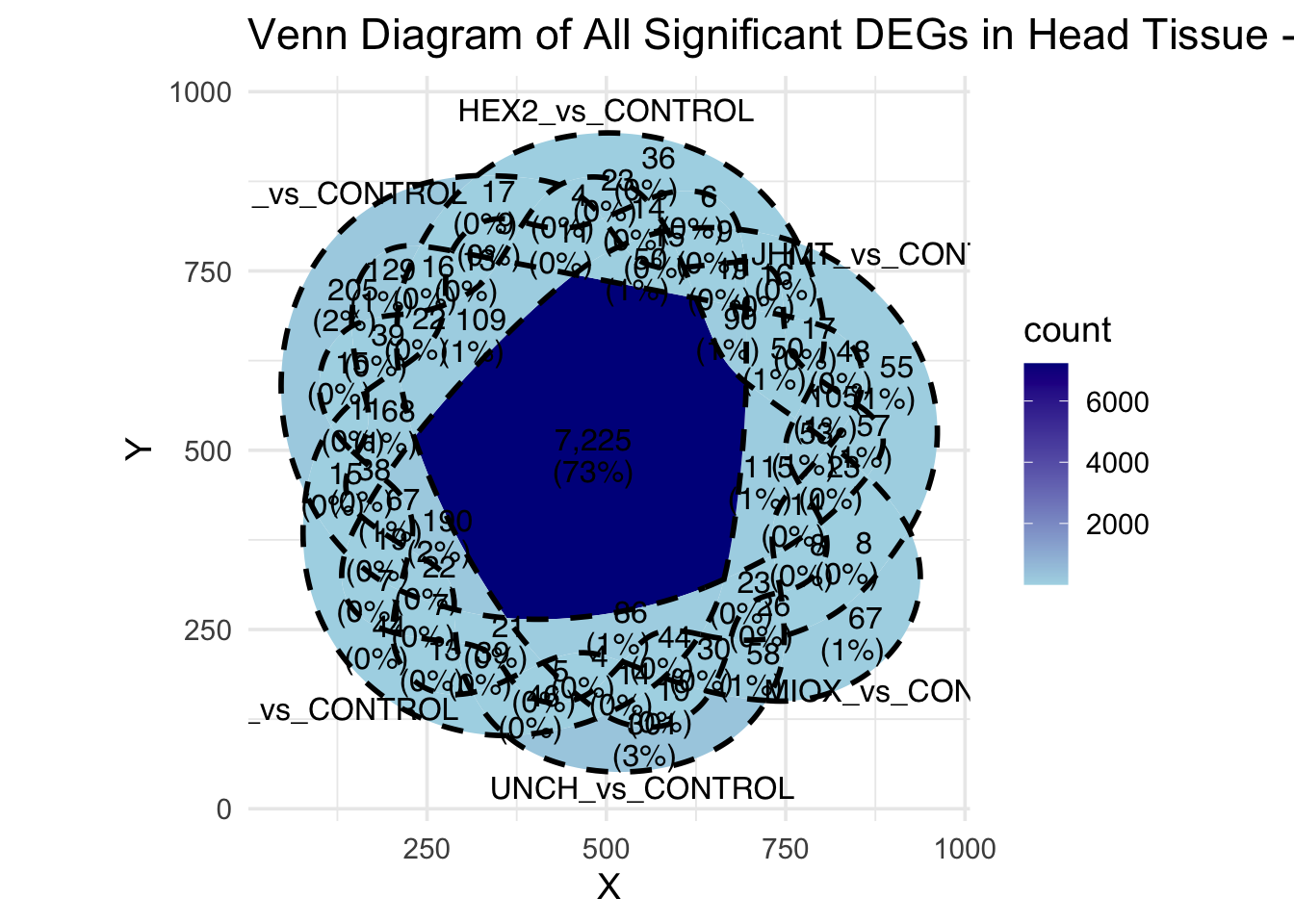
# Run the UpSet plot for Head Upregulated DEGs
display_upset_plot(venn_data_up, "UpSet Plot of Head Upregulated DEGs - RNAi Contrasts")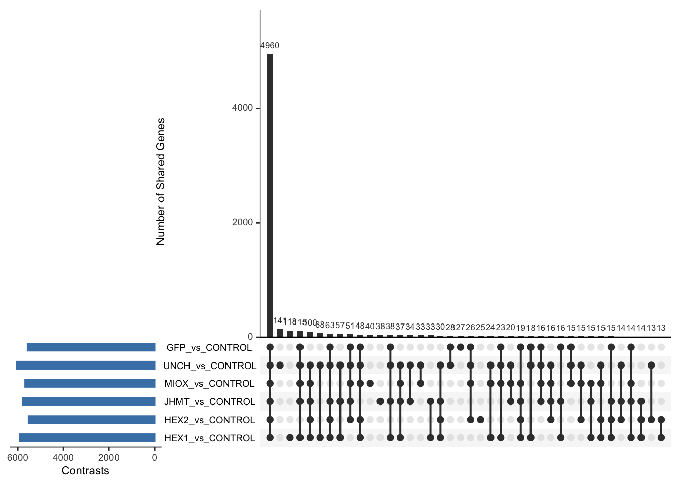
# Run the UpSet plot for Head Downregulated DEGs
display_upset_plot(venn_data_down, "UpSet Plot of Head Downregulated DEGs - RNAi Contrasts")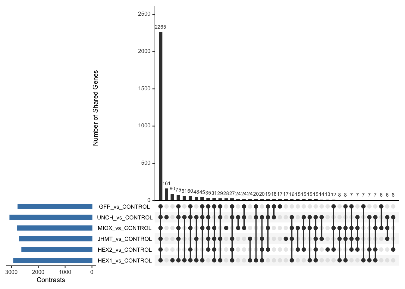
# Run the UpSet plot for Head Upregulated DEGs
display_upset_plot(venn_data_down, "UpSet Plot of All Significant DEGs in Head Tissue - RNAi Contrasts")
Thorax tissue
saveDir <- paste0(workDir,"/DEG_results/RNAi/Thorax_control_no_rRNA")
dir.create(saveDir)
### Prepare Sample CSV file #####
samples <- read.delim(file.path(workDir, "list/RNAi/Thorax_RNAi_noninjectedsample_list.csv"), sep = ",", row.names = 1, header = TRUE)
files <- file.path(workDir, "readcounts/RNAi/", samples$Tissue, samples$Filename)
names(files) <- row.names(samples)
if (all(file.exists(files))) {
message("All the files exist!")
} else {
warning("Some files are missing!")
}All the files exist!### **Standardized Count Matrix Creation**
# Extract all gene lists first
gene_lists <- map(files, function(sample) {
fread(sample, sep = "\t", header = FALSE)[, 1] # Extract Gene IDs (column 1)
})
# Get a unique set of all gene IDs across all samples
all_genes <- unique(unlist(gene_lists))
# Create a named list to store count data with standardized rows
cts_list <- map(files, function(sample) {
data_count <- fread(sample, sep = "\t", header = FALSE)
col_name <- gsub("_counts.txt", "", basename(sample)) # Clean sample name
# Convert to data frame with correct column names
data_count <- setNames(data.frame(data_count[, 1:2]), c("GeneID", col_name))
# Ensure all gene IDs are present (fill missing values with 0)
data_count <- full_join(data.frame(GeneID = all_genes), data_count, by = "GeneID") %>%
mutate(across(where(is.numeric), ~ replace_na(., 0))) # Fill NA with 0
return(data_count)
})
# Merge all samples based on GeneID
cts <- reduce(cts_list, full_join, by = "GeneID")
# Convert to matrix for DESeq2
cts_matrix <- as.matrix(cts[, -1]) # Remove GeneID column for count matrix
rownames(cts_matrix) <- cts$GeneID # Set GeneID as rownames
rm(cts_list) # Free memoryWhile for bulk RNAseq on head and thorax for all species, the DEGs model was made between isolated and crowded individuals (with isolated as the reference state), here, the DEG analysis will be carried between GFP knock-down nymphs (as reference state) vs Hexamerins / Juvenile Hormones / Inositol / Uncharacterized proteins.
### Build DESeq2 Object
dds <- DESeqDataSetFromMatrix(countData = cts_matrix,
colData = samples,
design = ~ Gene)
dds$Gene <- relevel(dds$Gene, ref = "CONTROL")
smallestGroupSize <- 5
keep <- rowSums(counts(dds) >= 10) >= smallestGroupSize
dds <- dds[keep,]
loci_to_exclude <- readLines(file.path(workDir, "list/excluded_loci/gregaria_rrna_list.txt"))
dds <- dds[!(rownames(dds) %in% loci_to_exclude), ]
dds <- DESeq(dds)Normalization and PCA
# Plot PCA and investigate quality metrics
vsd <- vst(dds, blind = TRUE)
# Perform PCA
pca_data <- plotPCA(vsd, intgroup = c("Tissue", "Gene"), returnData = TRUE)
# Define colors for genes (slightly transparent) and shapes for tissues
gene_colors <- scale_color_manual(values = alpha(brewer.pal(n = length(unique(pca_data$Gene)), name = "Set1"), 0.8)) # Points are transparent
tissue_shapes <- scale_shape_manual(values = seq(15, 15 + length(unique(pca_data$Tissue))))
# **PCA without labels**
p_pca_nolabel <- ggplot(pca_data, aes(x = PC1, y = PC2, color = Gene, shape = Tissue)) +
geom_point(size = 4) +
gene_colors +
tissue_shapes +
theme_bw() +
theme(legend.title = element_blank(),
legend.text = element_text(face = "bold", size = 14),
axis.text = element_text(size = 12),
axis.title = element_text(size = 14)) +
ggtitle("PCA of All Tissues (No Labels)", subtitle = "Tissues differentiated by shape, Genes by color")
# Save PCA without labels
ggsave(paste0(saveDir, "/PCA_Tissue_Gene_NoLabel.png"), plot = p_pca_nolabel, width = 10, height = 10, dpi = 600, device = "png")
# **PCA with labels**
p_pca_label <- ggplot(pca_data, aes(x = PC1, y = PC2, color = Gene, shape = Tissue)) +
geom_point(size = 4) +
geom_text_repel(aes(label = name), size = 4, color = "black", max.overlaps = 20) + # Labels are fully visible
gene_colors +
tissue_shapes +
theme_bw() +
theme(legend.title = element_blank(),
legend.text = element_text(face = "bold", size = 14),
axis.text = element_text(size = 12),
axis.title = element_text(size = 14)) +
ggtitle("PCA of All Tissues (With Labels)", subtitle = "Tissues differentiated by shape, Genes by color")
# Save PCA with labels
ggsave(paste0(saveDir, "/PCA_Tissue_Gene_Label.png"), plot = p_pca_label, width = 10, height = 10, dpi = 600, device = "png")
# **Return plots for knitr/RMarkdown**
list(NoLabel = p_pca_nolabel, WithLabel = p_pca_label)$NoLabel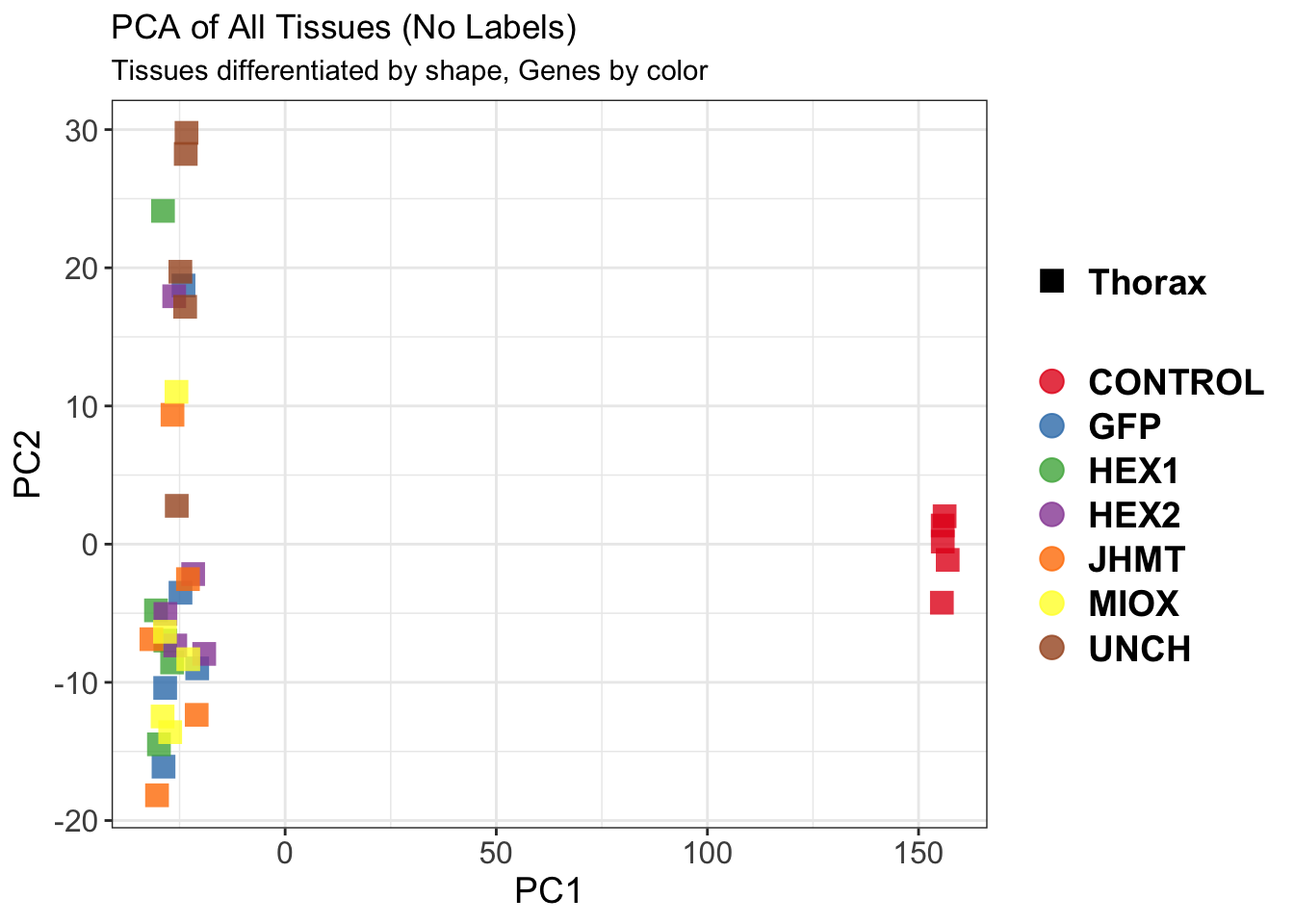
| Version | Author | Date |
|---|---|---|
| b540a1e | Maeva TECHER | 2025-02-27 |
$WithLabel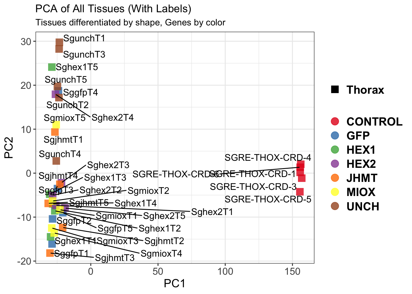
| Version | Author | Date |
|---|---|---|
| b540a1e | Maeva TECHER | 2025-02-27 |
The PCA plot shows clear distinction between tissue types, while gene silencing has a large variation within each tissue, and presents no distinct clear groupings for a single gene.
SVA
### SVA analysis to control for technical variation
dat <- counts(dds, normalized = TRUE)
idx <- rowMeans(dat) > 1
dat <- dat[idx, ]
mod <- model.matrix(~ Gene, colData(dds))
mod0 <- model.matrix(~ 1, colData(dds))
svseq <- svaseq(dat, mod, mod0)Number of significant surrogate variables is: 7
Iteration (out of 5 ):1 2 3 4 5 sva_plots <- create_sva_plots(svseq, dds, saveDir, intgroup = c("Tissue", "Gene"), max_sv = 6)
# Show stripcharts in the report
sva_plots$Stripcharts[[1]] # Show first stripchart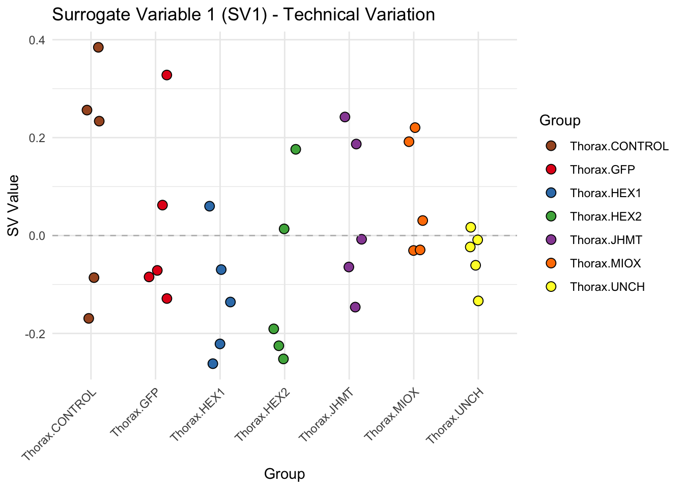
| Version | Author | Date |
|---|---|---|
| b540a1e | Maeva TECHER | 2025-02-27 |
sva_plots$Stripcharts[[2]] # Show second stripchart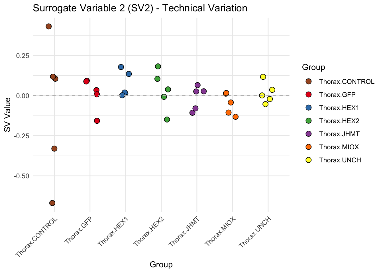
| Version | Author | Date |
|---|---|---|
| b540a1e | Maeva TECHER | 2025-02-27 |
sva_plots$Stripcharts[[3]] # Show third stripchart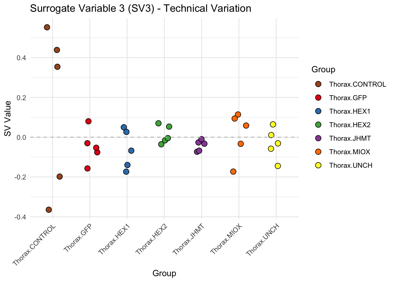
| Version | Author | Date |
|---|---|---|
| b540a1e | Maeva TECHER | 2025-02-27 |
sva_plots$Stripcharts[[4]] 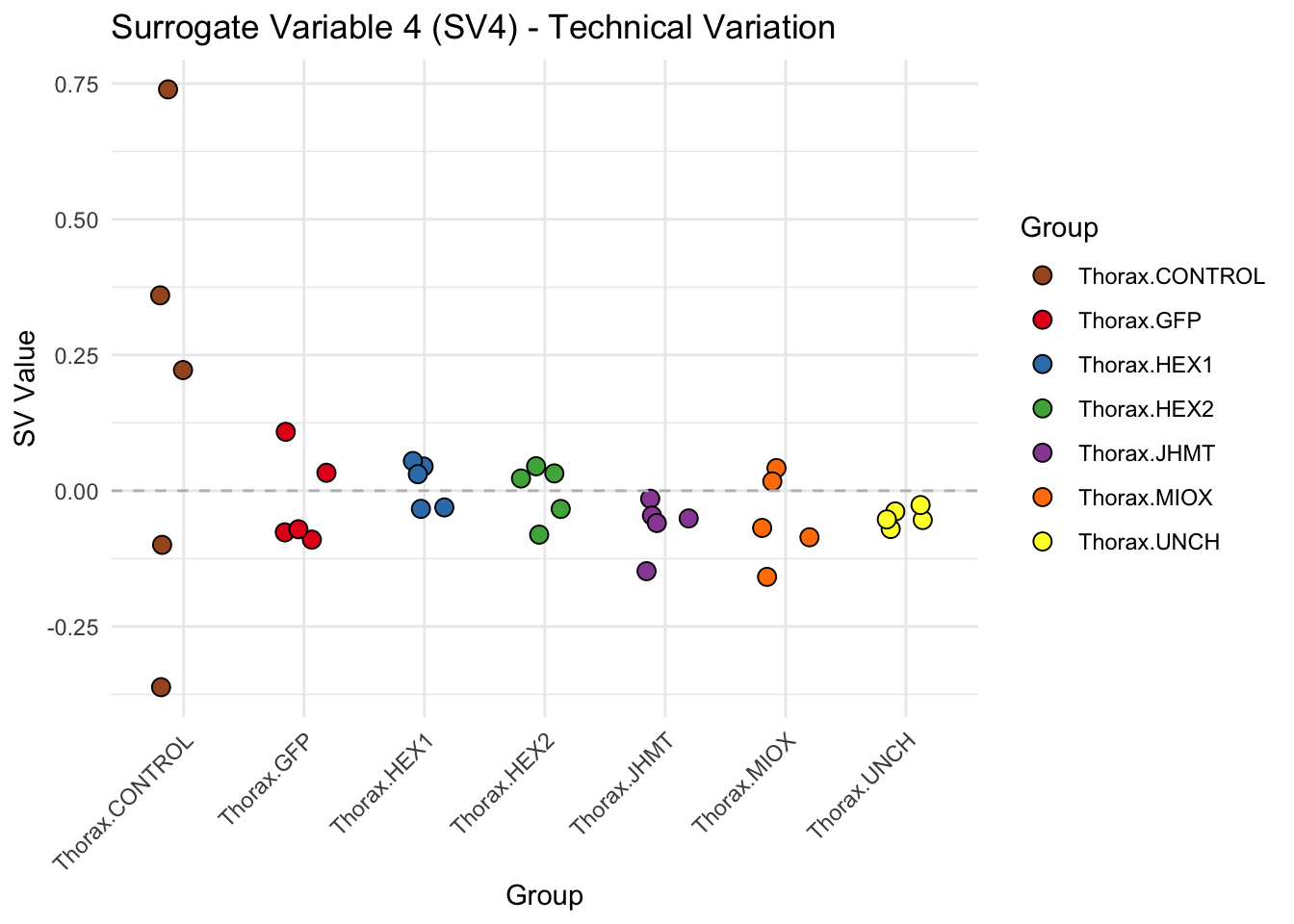
| Version | Author | Date |
|---|---|---|
| b540a1e | Maeva TECHER | 2025-02-27 |
sva_plots$Stripcharts[[5]]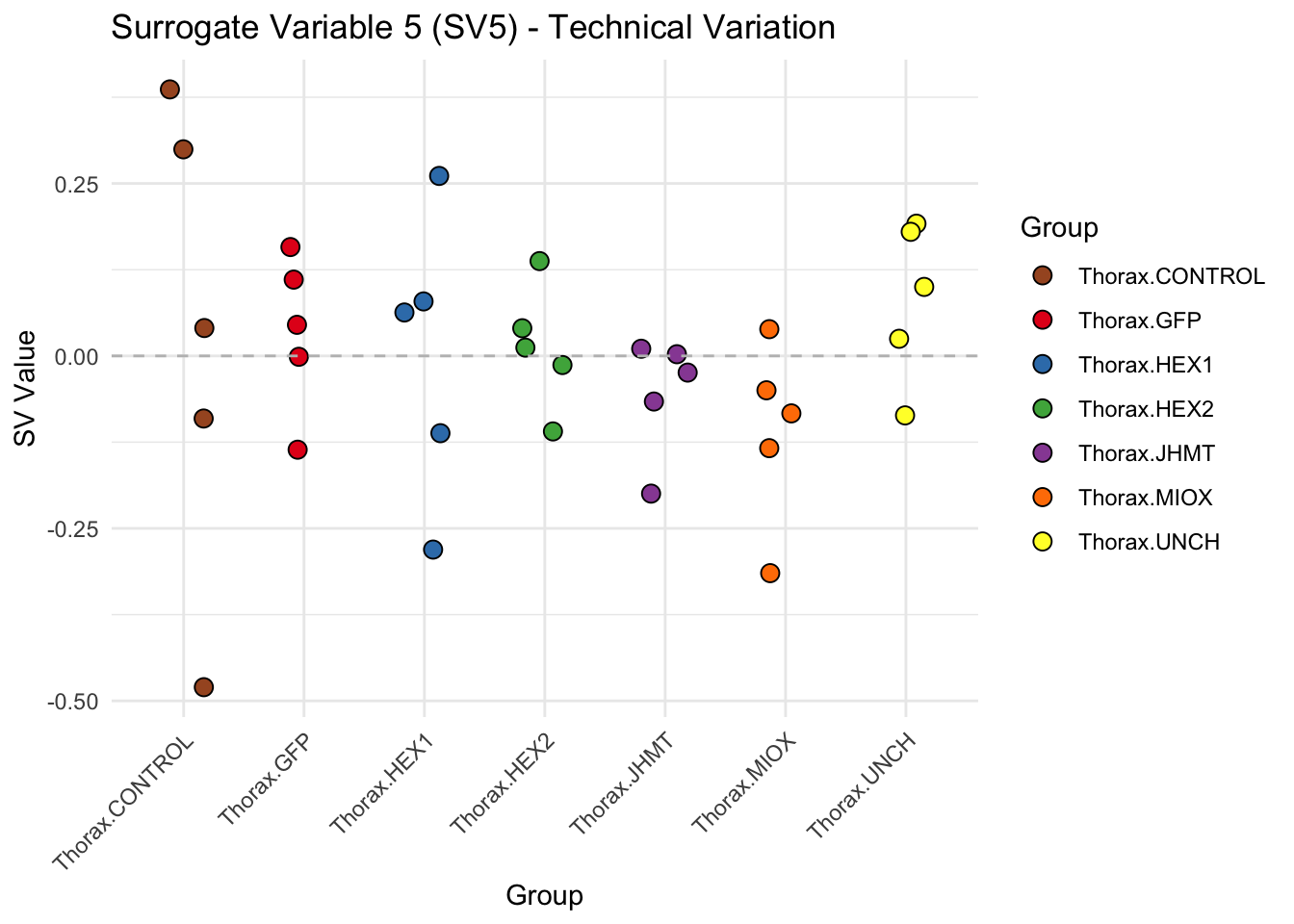
| Version | Author | Date |
|---|---|---|
| b540a1e | Maeva TECHER | 2025-02-27 |
sva_plots$Stripcharts[[6]] 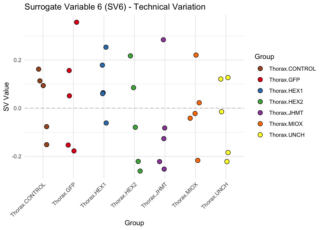
| Version | Author | Date |
|---|---|---|
| b540a1e | Maeva TECHER | 2025-02-27 |
# Show scatter plots in the report
sva_plots$ScatterPlots[["1_2"]] # Show SV1 vs SV2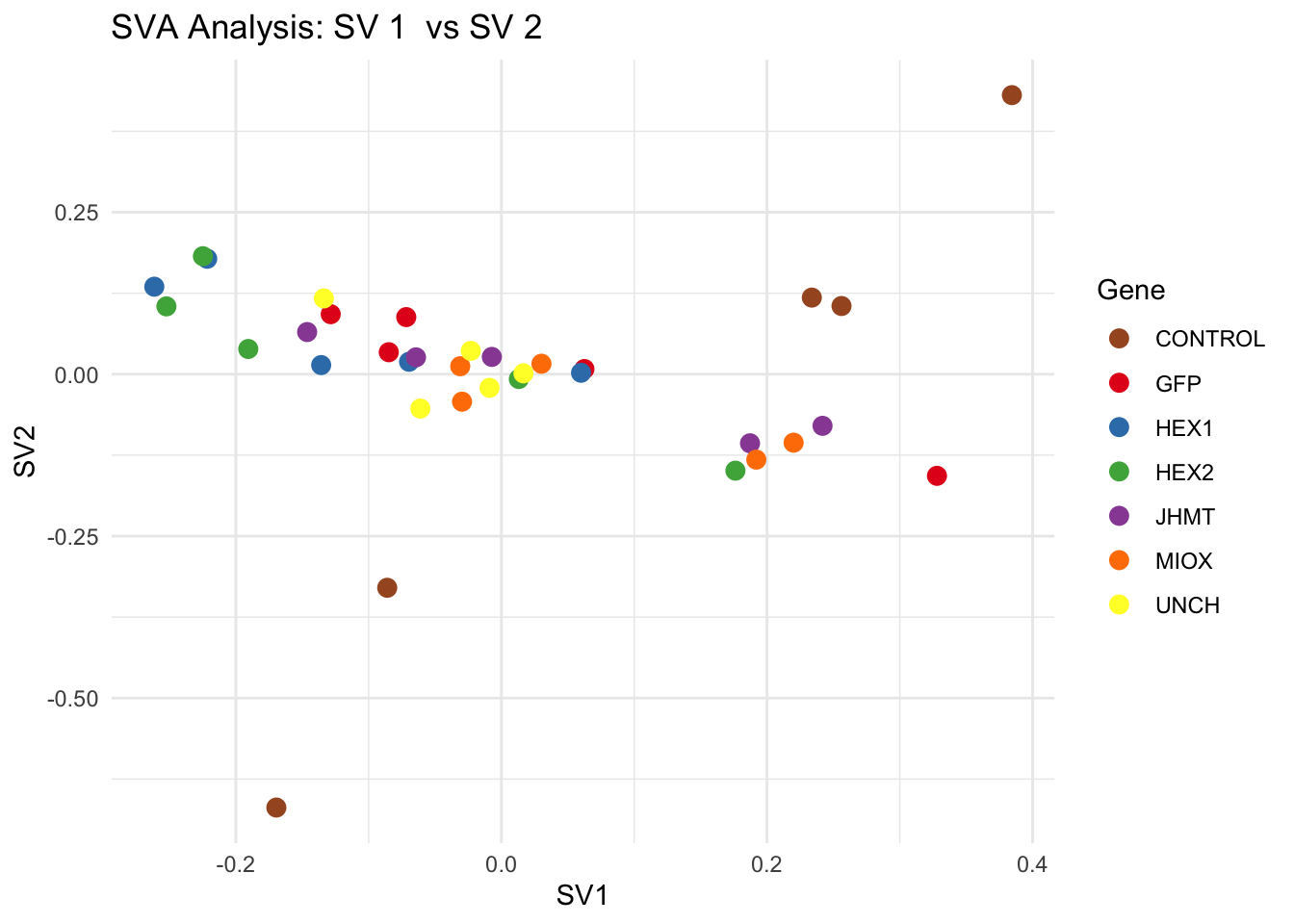
| Version | Author | Date |
|---|---|---|
| b540a1e | Maeva TECHER | 2025-02-27 |
sva_plots$ScatterPlots[["1_3"]] # Show SV1 vs SV3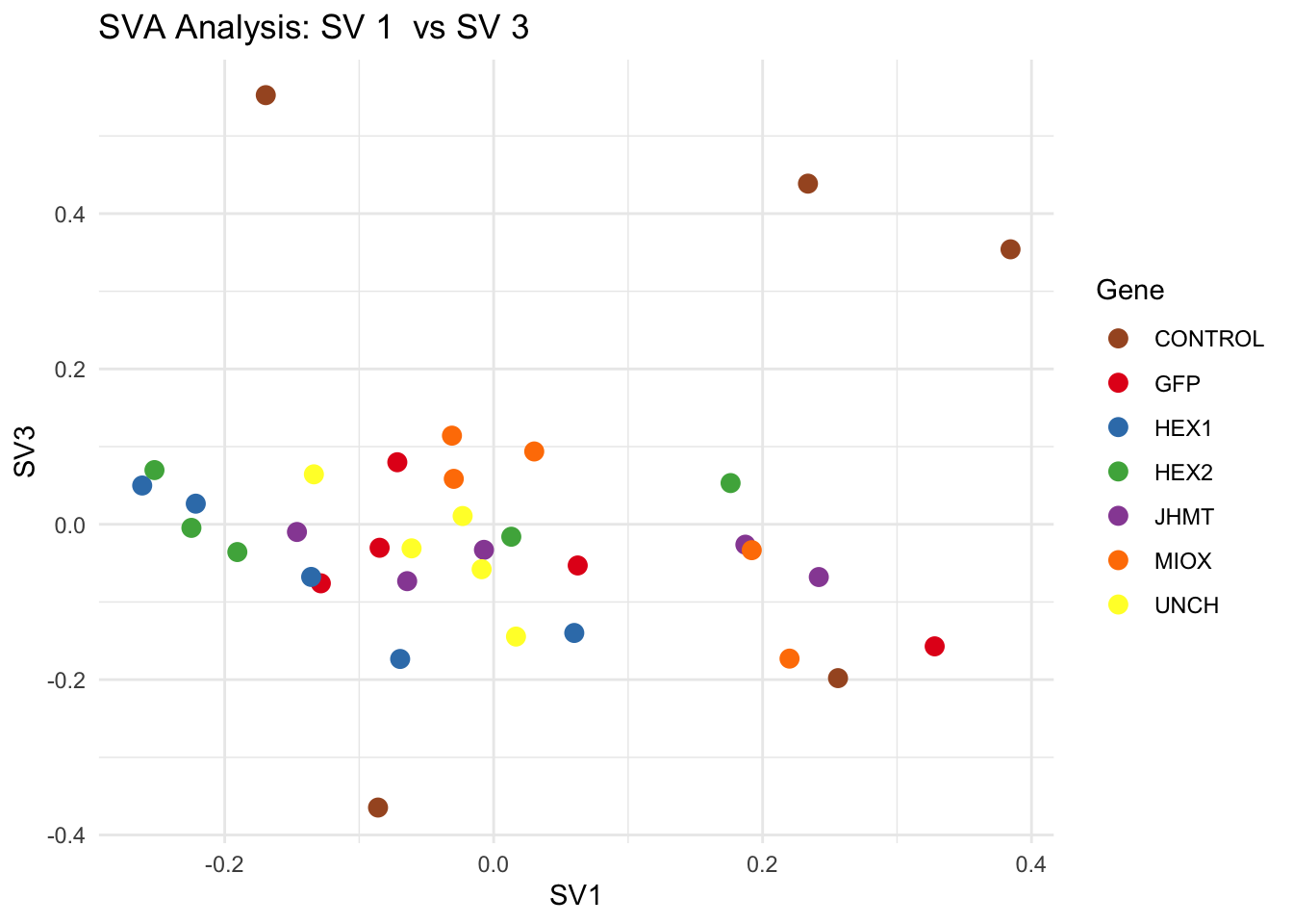
| Version | Author | Date |
|---|---|---|
| b540a1e | Maeva TECHER | 2025-02-27 |
sva_plots$ScatterPlots[["2_3"]] # Show SV2 vs SV3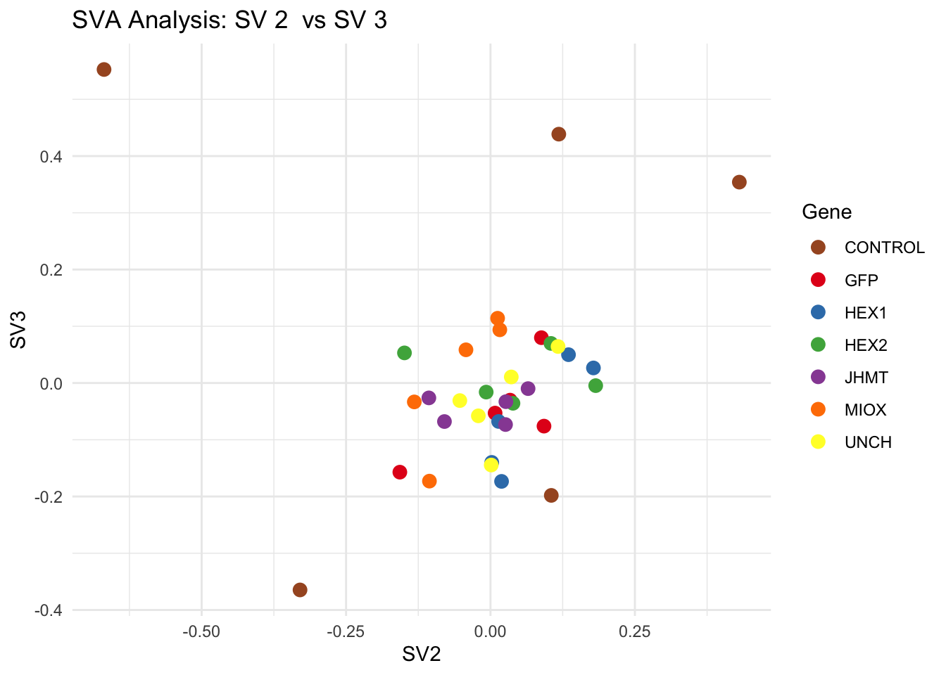
| Version | Author | Date |
|---|---|---|
| b540a1e | Maeva TECHER | 2025-02-27 |
SV1 is clearly showing an effect of tissue. We rerun the
DESeq2 model but this time including the surrogate variable
SV2 and SV3 as a covariates only, as we know that the modeled variation
is more likely explained by tissue and gene variation rather than batch
effects.
ddssva <- dds
ddssva$SV1 <- svseq$sv[,1]
ddssva$SV2 <- svseq$sv[,2]
ddssva$SV3 <- svseq$sv[,3]
ddssva$SV4 <- svseq$sv[,4]
ddssva$SV5 <- svseq$sv[,5]
ddssva$SV6 <- svseq$sv[,6]
design(ddssva) <- ~ SV1 + SV2 + SV3 + SV4 + SV5 + SV6 + Gene
ddssva$Gene <- relevel(ddssva$Gene, ref = "CONTROL")
smallestGroupSize <- 5
keep <- rowSums(counts(ddssva) >= 10) >= smallestGroupSize
ddssva <- ddssva[keep,]
ddssva <- DESeq(ddssva)
ddssva <- ddssva[which(mcols(ddssva)$betaConv),] # remove non converging rows
### Extract results
message("Available contrasts are: ", paste(resultsNames(ddssva), collapse = ", "))
hex1 <- results(ddssva, contrast = c("Gene", "HEX1", "CONTROL"), alpha = 0.05)
hex2 <- results(ddssva, contrast = c("Gene", "HEX2", "CONTROL"), alpha = 0.05)
jhmt <- results(ddssva, contrast = c("Gene", "JHMT", "CONTROL"), alpha = 0.05)
miox <- results(ddssva, contrast = c("Gene", "MIOX", "CONTROL"), alpha = 0.05)
unch <- results(ddssva, contrast = c("Gene", "UNCH", "CONTROL"), alpha = 0.05)
gfp <- results(ddssva, contrast = c("Gene", "GFP", "CONTROL"), alpha = 0.05)Volcano plots and Heatmaps
# Define contrast_sets
hex1_samples <- c("SGRE-THOX-CRD-1","SGRE-THOX-CRD-3","SGRE-THOX-CRD-4","SGRE-THOX-CRD-5",
"SGRE-THOX-CRD-6","SggfpT1","SggfpT2","SggfpT3","SggfpT4","SggfpT5",
"Sghex1T1","Sghex1T2","Sghex1T3","Sghex1T4","Sghex1T5")
hex2_samples <- c("SGRE-THOX-CRD-1","SGRE-THOX-CRD-3","SGRE-THOX-CRD-4","SGRE-THOX-CRD-5",
"SGRE-THOX-CRD-6","SggfpT1","SggfpT2","SggfpT3","SggfpT4","SggfpT5",
"Sghex2T1","Sghex2T2","Sghex2T3","Sghex2T4","Sghex2T5")
jhmt_samples <- c("SGRE-THOX-CRD-1","SGRE-THOX-CRD-3","SGRE-THOX-CRD-4","SGRE-THOX-CRD-5",
"SGRE-THOX-CRD-6","SggfpT1","SggfpT2","SggfpT3","SggfpT4","SggfpT5",
"SgjhmtT1","SgjhmtT2","SgjhmtT3","SgjhmtT4","SgjhmtT5")
miox_samples <- c("SGRE-THOX-CRD-1","SGRE-THOX-CRD-3","SGRE-THOX-CRD-4","SGRE-THOX-CRD-5",
"SGRE-THOX-CRD-6","SggfpT1","SggfpT2","SggfpT3","SggfpT4","SggfpT5",
"SgmioxT1","SgmioxT2","SgmioxT3","SgmioxT4","SgmioxT5")
unch_samples <- c("SGRE-THOX-CRD-1","SGRE-THOX-CRD-3","SGRE-THOX-CRD-4","SGRE-THOX-CRD-5",
"SGRE-THOX-CRD-6","SggfpT1","SggfpT2","SggfpT3","SggfpT4","SggfpT5",
"SgunchT1","SgunchT2","SgunchT3","SgunchT4","SgunchT5")
gfp_samples <- c("SGRE-THOX-CRD-1","SGRE-THOX-CRD-3","SGRE-THOX-CRD-4","SGRE-THOX-CRD-5",
"SGRE-THOX-CRD-6", "SggfpT1","SggfpT2","SggfpT3","SggfpT4","SggfpT5")
# Run full analysis
hex1_plots <- visualize_data_nopng(hex1, "HEX1_vs_CONTROL", hex1_samples)
hex2_plots <- visualize_data_nopng(hex2, "HEX2_vs_CONTROL", hex2_samples)
jhmt_plots <- visualize_data_nopng(jhmt, "JHMT_vs_CONTROL", jhmt_samples)
miox_plots <- visualize_data_nopng(miox, "MIOX_vs_CONTROL", miox_samples)
unch_plots <- visualize_data_nopng(unch, "UNCH_vs_CONTROL", unch_samples)
gfp_plots <- visualize_data_nopng(gfp, "GFP_vs_CONTROL", gfp_samples)
hex1_plots$volcano; hex1_plots$heatmap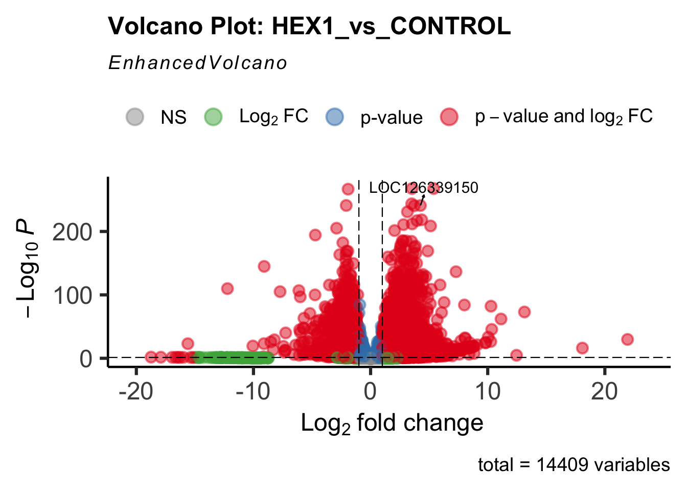
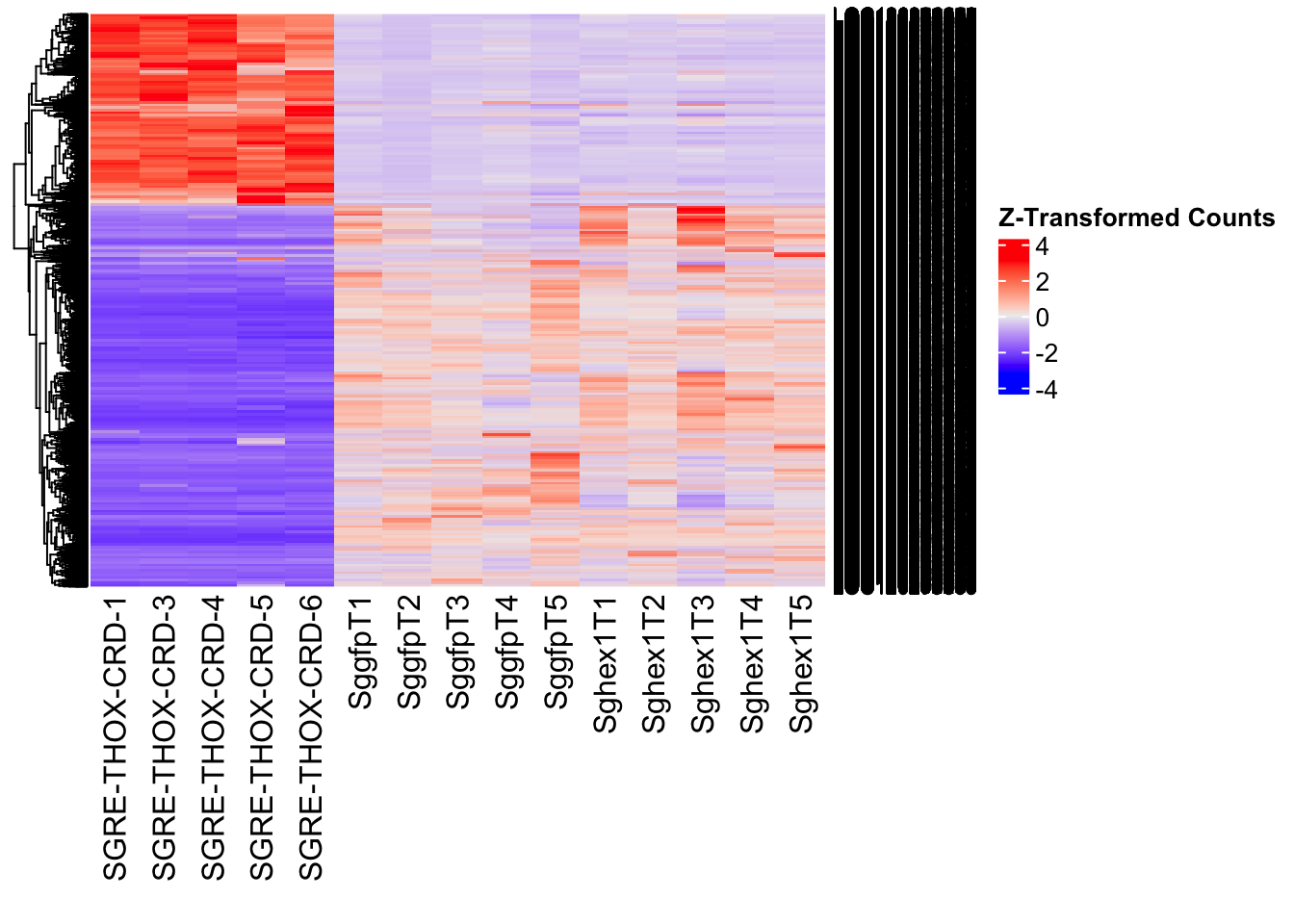
| Version | Author | Date |
|---|---|---|
| b540a1e | Maeva TECHER | 2025-02-27 |
hex2_plots$volcano; hex2_plots$heatmap
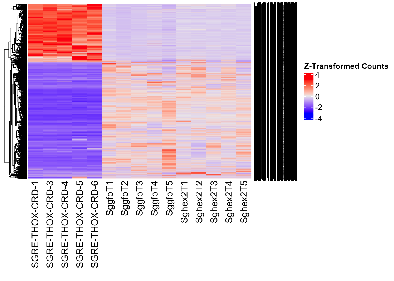
| Version | Author | Date |
|---|---|---|
| b540a1e | Maeva TECHER | 2025-02-27 |
jhmt_plots$volcano; jhmt_plots$heatmap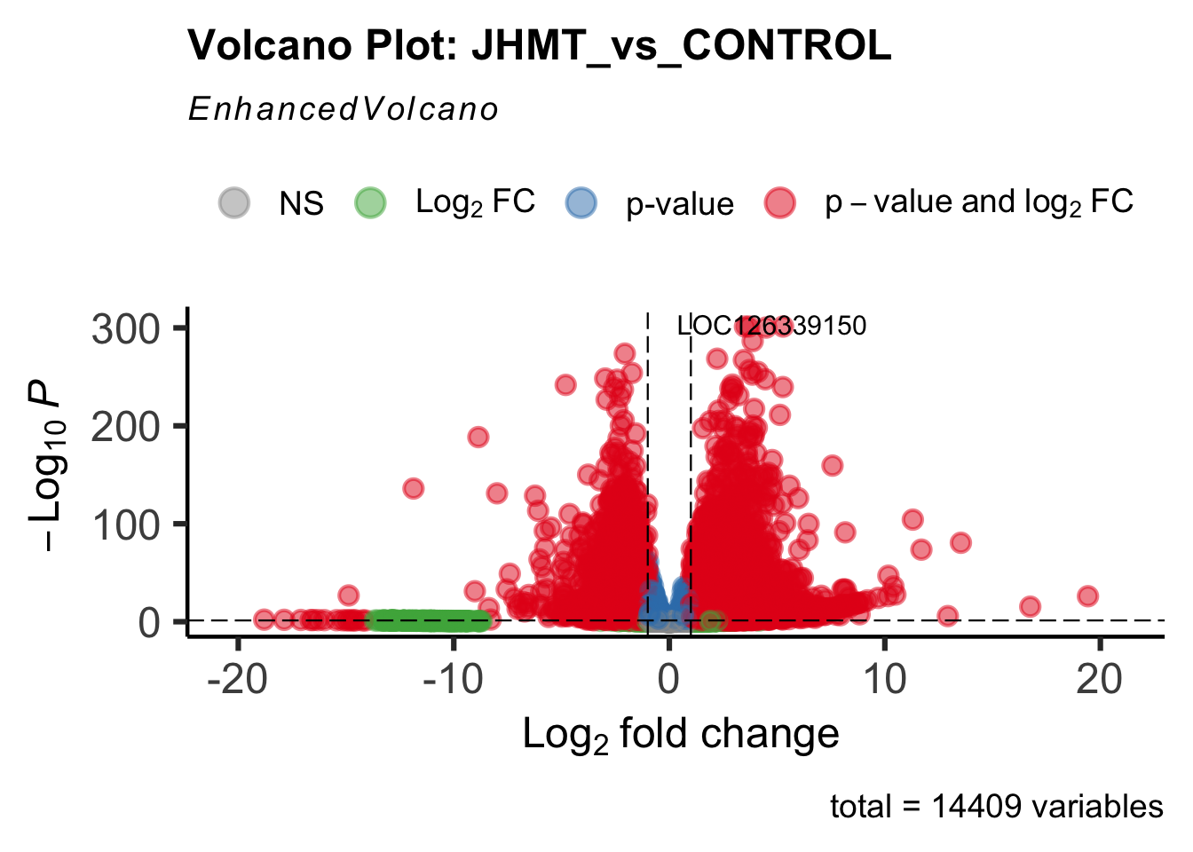
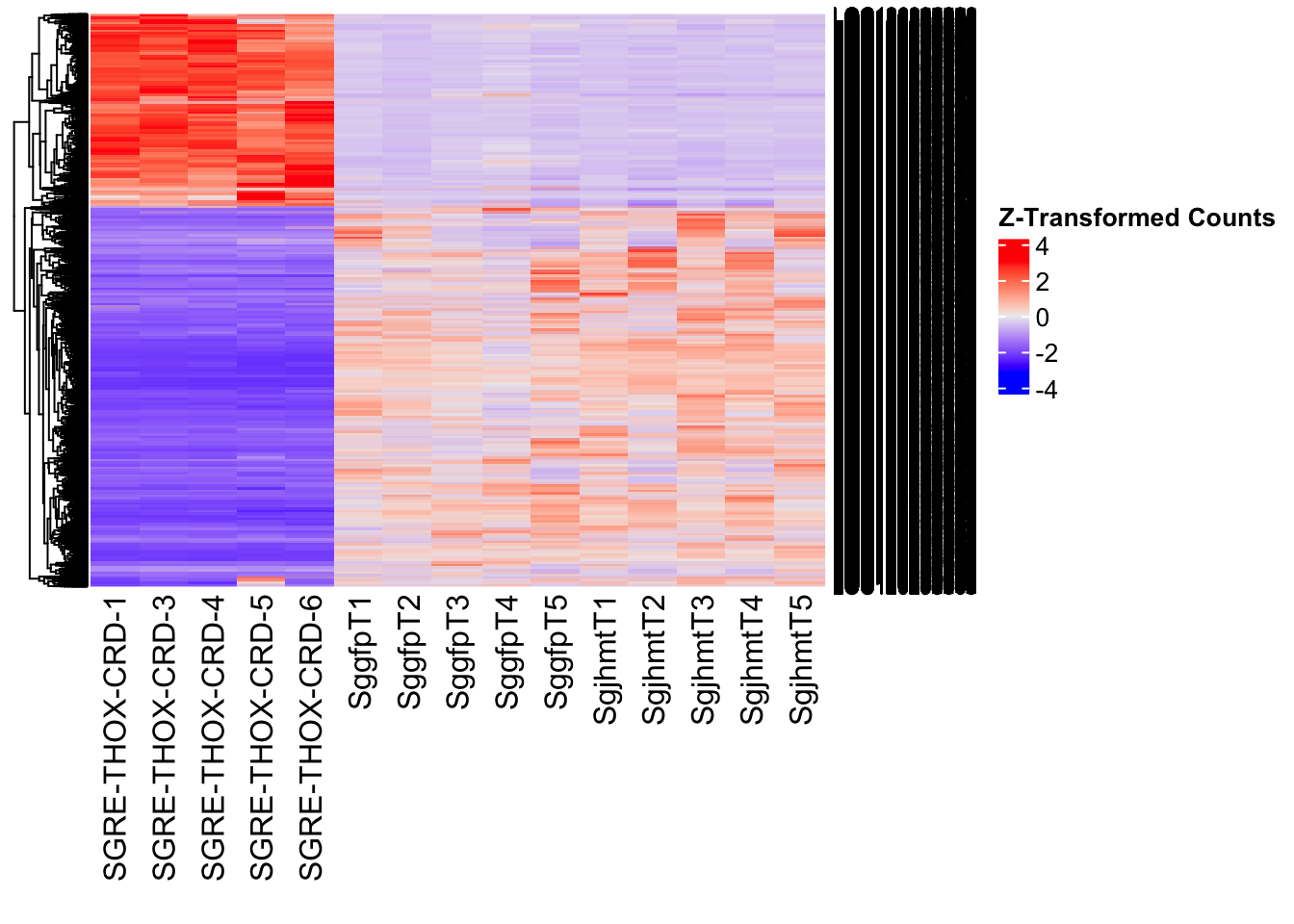
| Version | Author | Date |
|---|---|---|
| b540a1e | Maeva TECHER | 2025-02-27 |
miox_plots$volcano; miox_plots$heatmap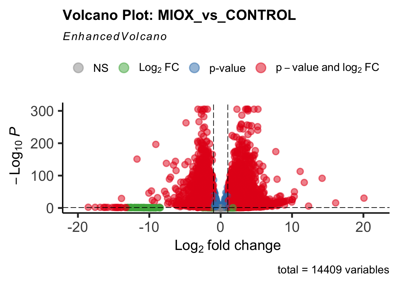
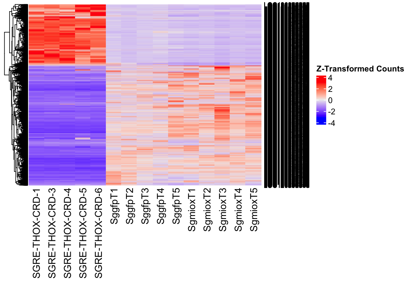
| Version | Author | Date |
|---|---|---|
| b540a1e | Maeva TECHER | 2025-02-27 |
unch_plots$volcano; unch_plots$heatmap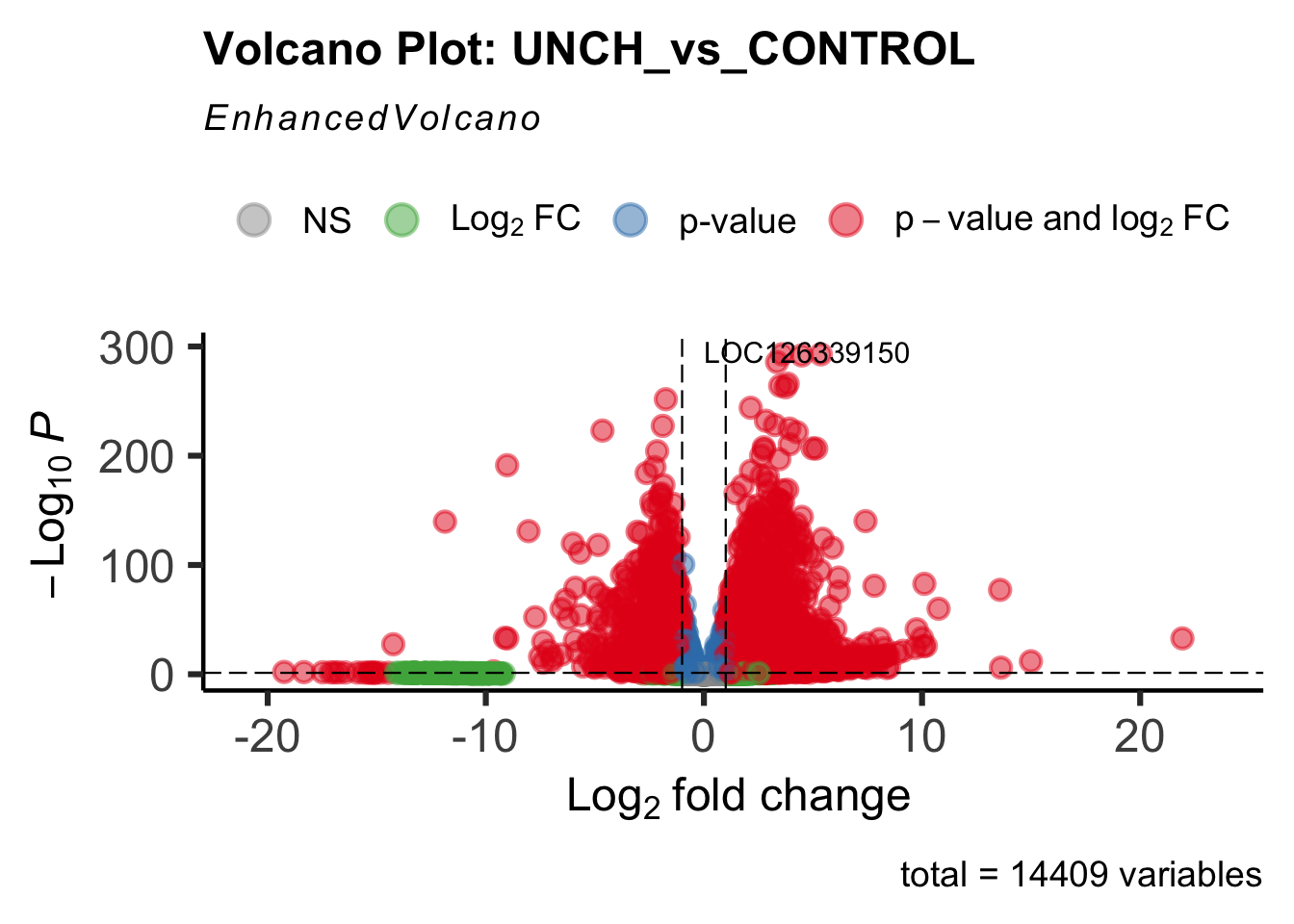
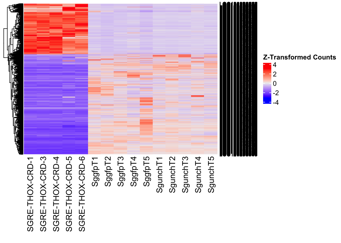
gfp_plots$volcano; gfp_plots$heatmap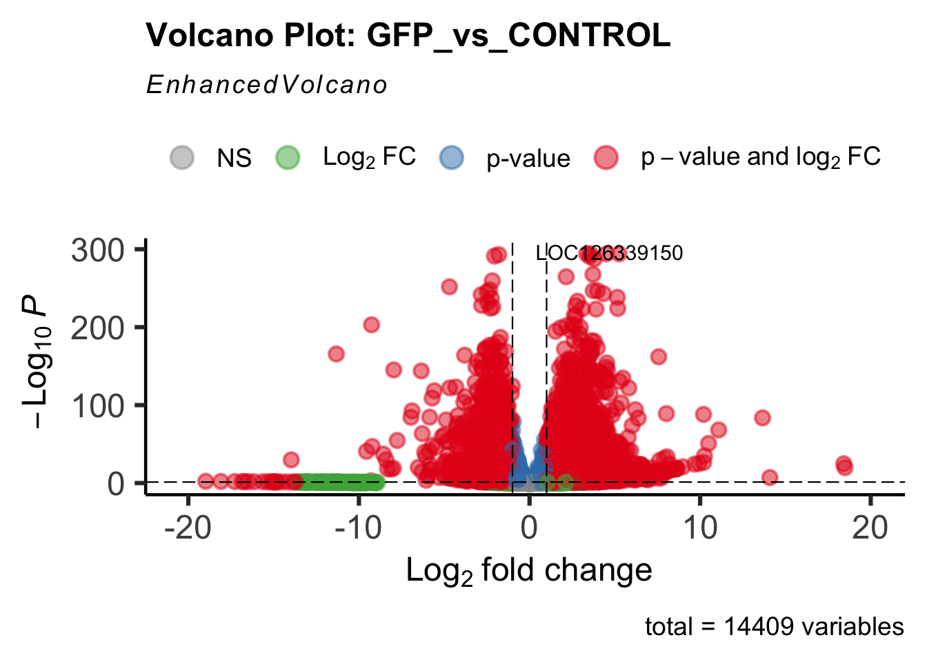
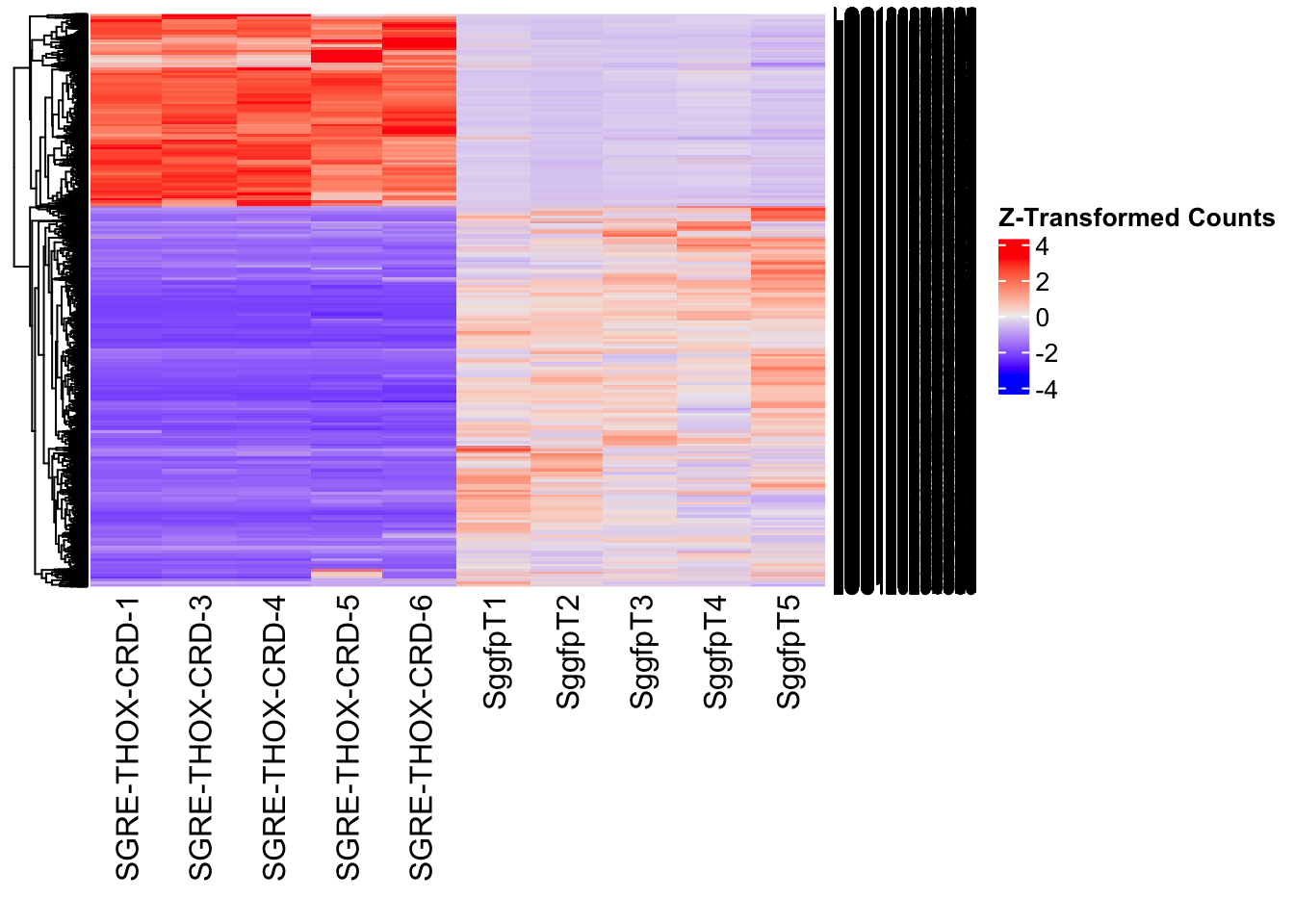
DEG tables
The following tables show the genes differentially expressed with at least an absolute log2fold change of > 1 considering Head tissues only. Considering GFP as the reference state, upregulated genes in knockdown treatment in red and downregulated genes in knockdown treatment in blue. You can search for a gene of interest by writting a LOCID or description in the search bar or sort by column.
# Generate tables for each contrast
table_hex1 <- generate_deg_table(ddssva, "Gene_HEX1_vs_CONTROL", allspecies_df)
out of 14409 with nonzero total read count
adjusted p-value < 0.05
LFC > 0 (up) : 6704, 47%
LFC < 0 (down) : 4208, 29%
outliers [1] : 0, 0%
low counts [2] : 0, 0%
(mean count < 3)
[1] see 'cooksCutoff' argument of ?results
[2] see 'independentFiltering' argument of ?resultsTotal DEGs p-value < 0.05 and absolute logFoldChange > 1: 8162LFC > 1 (up) : 5437 (66.61%)LFC < -1 (down) : 2725 (33.39%)table_hex1$kable_tabletable_hex2 <- generate_deg_table(ddssva, "Gene_HEX2_vs_CONTROL", allspecies_df)
out of 14409 with nonzero total read count
adjusted p-value < 0.05
LFC > 0 (up) : 6686, 46%
LFC < 0 (down) : 4250, 29%
outliers [1] : 0, 0%
low counts [2] : 0, 0%
(mean count < 3)
[1] see 'cooksCutoff' argument of ?results
[2] see 'independentFiltering' argument of ?resultsTotal DEGs p-value < 0.05 and absolute logFoldChange > 1: 7953LFC > 1 (up) : 5320 (66.89%)LFC < -1 (down) : 2633 (33.11%)table_hex2$kable_tabletable_jhmt <- generate_deg_table(ddssva, "Gene_JHMT_vs_CONTROL", allspecies_df)
out of 14409 with nonzero total read count
adjusted p-value < 0.05
LFC > 0 (up) : 7005, 49%
LFC < 0 (down) : 4332, 30%
outliers [1] : 0, 0%
low counts [2] : 0, 0%
(mean count < 3)
[1] see 'cooksCutoff' argument of ?results
[2] see 'independentFiltering' argument of ?resultsTotal DEGs p-value < 0.05 and absolute logFoldChange > 1: 8566LFC > 1 (up) : 5685 (66.37%)LFC < -1 (down) : 2881 (33.63%)table_jhmt$kable_tabletable_miox <- generate_deg_table(ddssva, "Gene_MIOX_vs_CONTROL", allspecies_df)
out of 14409 with nonzero total read count
adjusted p-value < 0.05
LFC > 0 (up) : 7179, 50%
LFC < 0 (down) : 4400, 31%
outliers [1] : 0, 0%
low counts [2] : 0, 0%
(mean count < 3)
[1] see 'cooksCutoff' argument of ?results
[2] see 'independentFiltering' argument of ?resultsTotal DEGs p-value < 0.05 and absolute logFoldChange > 1: 8720LFC > 1 (up) : 5778 (66.26%)LFC < -1 (down) : 2942 (33.74%)table_miox$kable_tabletable_unch <- generate_deg_table(ddssva, "Gene_UNCH_vs_CONTROL", allspecies_df)
out of 14409 with nonzero total read count
adjusted p-value < 0.05
LFC > 0 (up) : 6666, 46%
LFC < 0 (down) : 4259, 30%
outliers [1] : 0, 0%
low counts [2] : 0, 0%
(mean count < 3)
[1] see 'cooksCutoff' argument of ?results
[2] see 'independentFiltering' argument of ?resultsTotal DEGs p-value < 0.05 and absolute logFoldChange > 1: 8007LFC > 1 (up) : 5321 (66.45%)LFC < -1 (down) : 2686 (33.55%)table_unch$kable_tabletable_gfp <- generate_deg_table(ddssva, "Gene_GFP_vs_CONTROL", allspecies_df)
out of 14409 with nonzero total read count
adjusted p-value < 0.05
LFC > 0 (up) : 6898, 48%
LFC < 0 (down) : 4311, 30%
outliers [1] : 0, 0%
low counts [2] : 0, 0%
(mean count < 3)
[1] see 'cooksCutoff' argument of ?results
[2] see 'independentFiltering' argument of ?resultsTotal DEGs p-value < 0.05 and absolute logFoldChange > 1: 8322LFC > 1 (up) : 5524 (66.38%)LFC < -1 (down) : 2798 (33.62%)table_gfp$kable_tableSummary and Overlap
# Summarize DEGs for all contrasts
deg_summary <- bind_rows(
summarize_deg_counts(table_hex1, "HEX1 vs CONTROL"),
summarize_deg_counts(table_hex2, "HEX2 vs CONTROL"),
summarize_deg_counts(table_jhmt, "JHMT vs CONTROL"),
summarize_deg_counts(table_miox, "MIOX vs CONTROL"),
summarize_deg_counts(table_unch, "UNCH vs CONTROL"),
summarize_deg_counts(table_gfp, "GFP vs CONTROL")
)
# Display table using kable with styling
deg_summary %>%
kable("html", escape = FALSE, col.names = gsub("_", " ", names(.))) %>%
kable_styling("striped", full_width = TRUE) %>%
column_spec(2, color = "red", bold = TRUE) %>% # Upregulated in red
column_spec(3, color = "blue", bold = TRUE) %>% # Downregulated in blue
add_header_above(c("Summary of DEGs" = 3)) %>%
row_spec(0, bold = TRUE)| Contrast | Upregulated | Downregulated |
|---|---|---|
| HEX1 vs CONTROL | 5393 | 2705 |
| HEX2 vs CONTROL | 5277 | 2622 |
| JHMT vs CONTROL | 5633 | 2864 |
| MIOX vs CONTROL | 5733 | 2924 |
| UNCH vs CONTROL | 5264 | 2675 |
| GFP vs CONTROL | 5467 | 2785 |
# Define the list of RNAi contrasts
contrast_list <- c("HEX1_vs_CONTROL", "HEX2_vs_CONTROL", "JHMT_vs_CONTROL",
"MIOX_vs_CONTROL", "UNCH_vs_CONTROL", "GFP_vs_CONTROL")
# Initialize empty lists for storing Head-specific DEGs for each contrast
venn_data_up <- list()
venn_data_down <- list()
venn_data_all <- list()
# Function to load Head-specific DEGs for a given set of contrasts
load_deg_contrasts_head <- function(contrast_list) {
degs_up <- list()
degs_down <- list()
degs_all <- list()
for (contrast in contrast_list) {
deg_file <- file.path(workDir, "DEG_results/RNAi/Thorax_control_no_rRNA/", contrast, paste0("DEG_sigresults_", contrast, ".csv"))
if (!file.exists(deg_file)) {
message(paste("File missing for contrast:", contrast))
next # Skip if the file doesn't exist
}
deg_data <- read.csv(deg_file, stringsAsFactors = FALSE)
# Convert row names to a column if necessary
if ("X" %in% colnames(deg_data)) {
colnames(deg_data)[colnames(deg_data) == "X"] <- "GeneID"
}
# Check if data is empty
if (nrow(deg_data) == 0) {
message(paste("No data for contrast:", contrast))
next
}
# Select significant DEGs (Up, Down, All)
degs_up[[contrast]] <- deg_data %>%
filter(padj < 0.05 & log2FoldChange >= 1) %>%
pull(GeneID) # Extract GeneID column
degs_down[[contrast]] <- deg_data %>%
filter(padj < 0.05 & log2FoldChange <= -1) %>%
pull(GeneID) # Extract GeneID column
degs_all[[contrast]] <- deg_data %>%
filter(padj < 0.05 & abs(log2FoldChange) >= 1) %>%
pull(GeneID) # Extract GeneID column
}
return(list(up = degs_up, down = degs_down, all = degs_all))
}
# Load DEG data for the defined contrasts (Head tissue only)
venn_data_contrasts <- load_deg_contrasts_head(contrast_list)
# Prepare the data for the Venn diagrams
venn_data_up <- venn_data_contrasts$up
venn_data_down <- venn_data_contrasts$down
venn_data_all <- venn_data_contrasts$all
# Display the Venn diagram and datatable for **Head Upregulated DEGs** across contrasts
display_ggvenn_plot(venn_data_up, "Venn Diagram of Thorax Upregulated DEGs - RNAi Contrasts")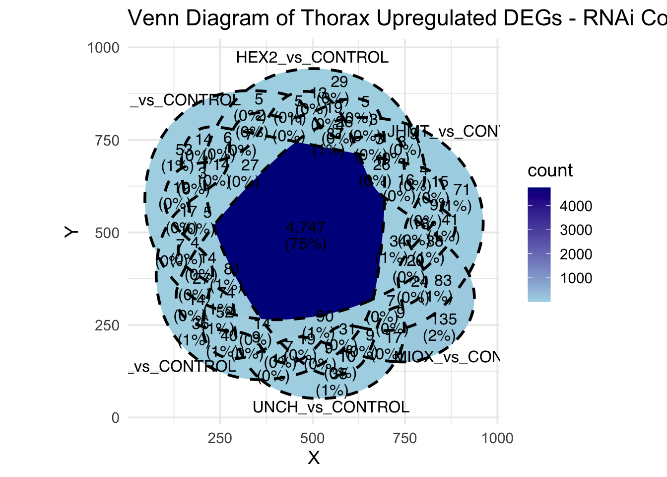
# Display the Venn diagram and datatable for **Head Downregulated DEGs** across contrasts
display_ggvenn_plot(venn_data_down, "Venn Diagram of Thorax Downregulated DEGs - RNAi Contrasts")
# Display the Venn diagram and datatable for **All Significant DEGs in Head Tissue**
display_ggvenn_plot(venn_data_all, "Venn Diagram of All Significant DEGs in Thorax Tissue - RNAi Contrasts")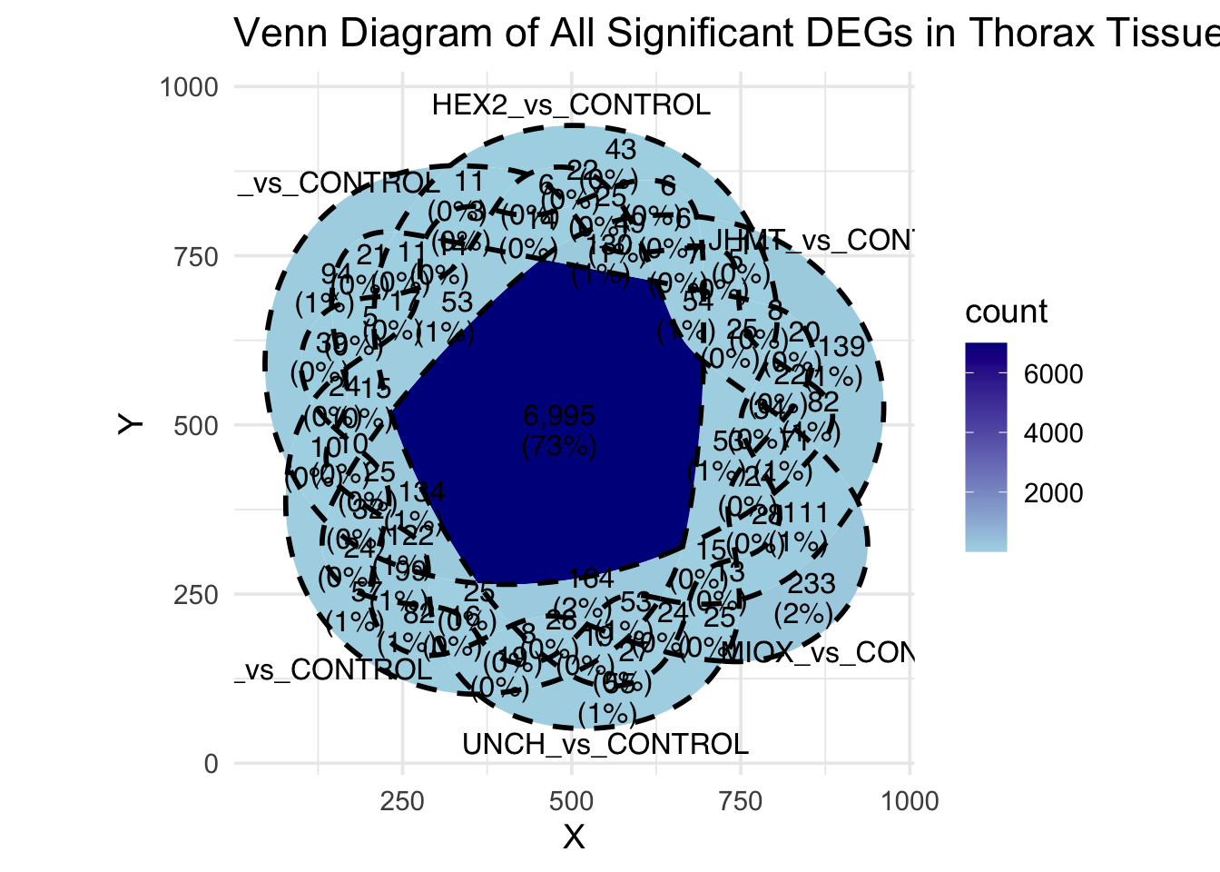
# Run the UpSet plot for Head Upregulated DEGs
display_upset_plot(venn_data_up, "UpSet Plot of Thorax Upregulated DEGs - RNAi Contrasts")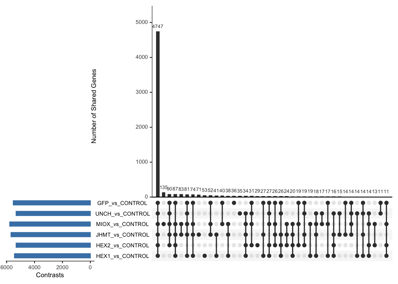
# Run the UpSet plot for Head Downregulated DEGs
display_upset_plot(venn_data_down, "UpSet Plot of Thorax Downregulated DEGs - RNAi Contrasts")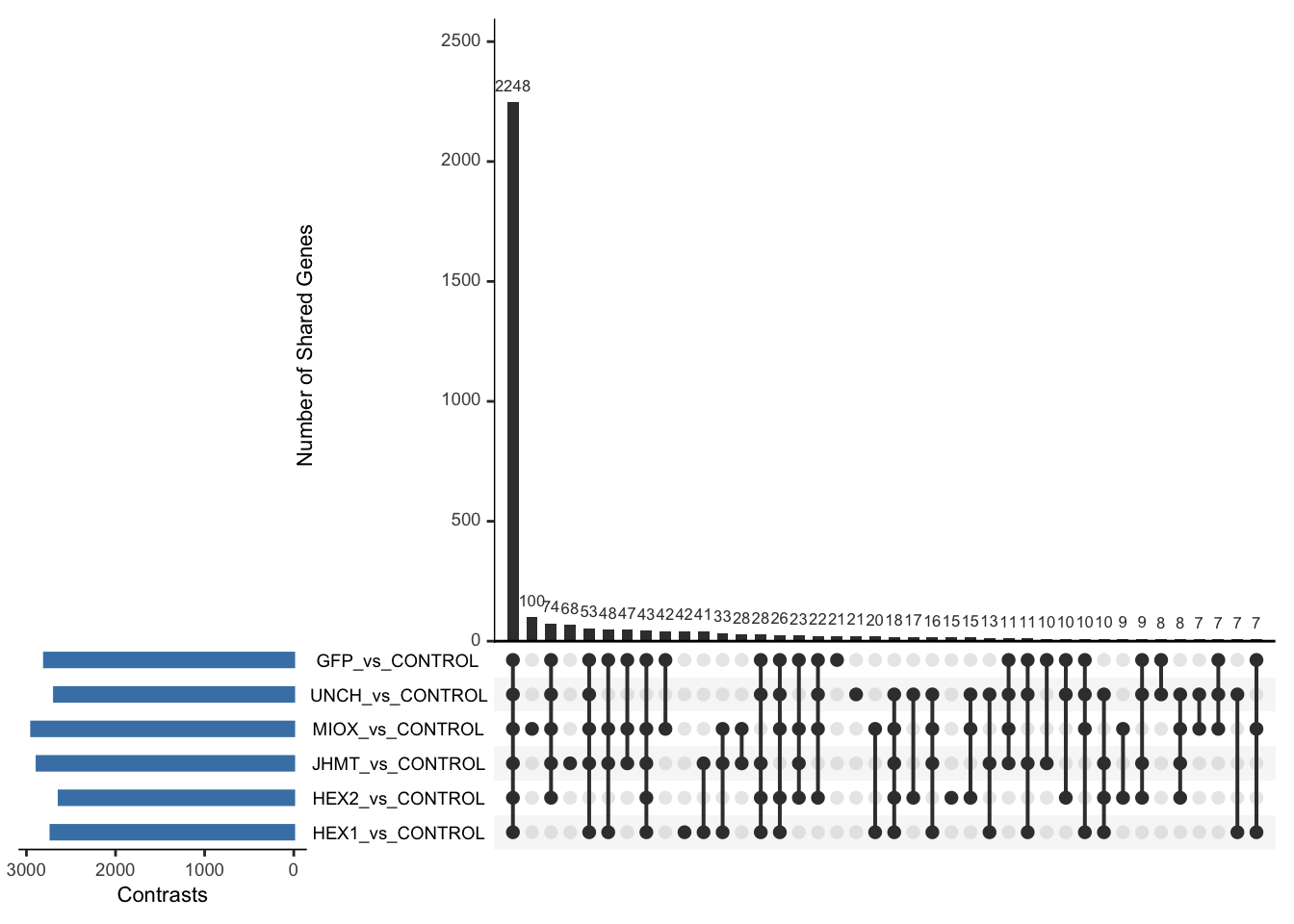
# Run the UpSet plot for Head Upregulated DEGs
display_upset_plot(venn_data_all, "UpSet Plot of All Significant DEGs in Thorax Tissue - RNAi Contrasts")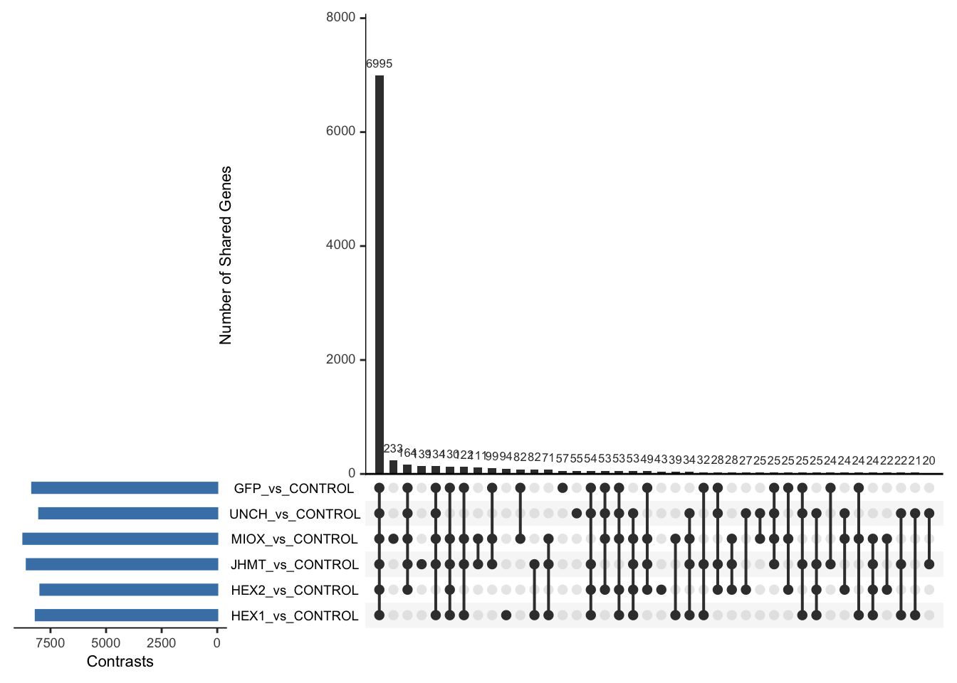
6. Comparison between GFP vs Crowded
All genes included
All tissue together
Minor changes here are made compared to the DESeq2
results regarding the importation of samples to transform into a
matrix.
Sample names are structured as follow: {Sg}{gene}{#} {Sg} = Schistocerca gregaria {gene} = gene abbreviation gfp, hex1, hex2, jhmt, miox and unch H/T{#} = biological replicate
saveDir <- paste0(workDir,"/DEG_results/RNAi/All_GFP")
dir.create(saveDir)
### Prepare Sample CSV file #####
samples <- read.delim(file.path(workDir, "list/RNAi/All_RNAi_GFPCRDsample_list.csv"), sep = ",", row.names = 1, header = TRUE)
files <- file.path(workDir, "readcounts/RNAi/", samples$Tissue, samples$Filename)
names(files) <- row.names(samples)
if (all(file.exists(files))) {
message("All the files exist!")
} else {
warning("Some files are missing!")
}All the files exist!### **Standardized Count Matrix Creation**
# Extract all gene lists first
gene_lists <- map(files, function(sample) {
fread(sample, sep = "\t", header = FALSE)[, 1] # Extract Gene IDs (column 1)
})
# Get a unique set of all gene IDs across all samples
all_genes <- unique(unlist(gene_lists))
# Create a named list to store count data with standardized rows
cts_list <- map(files, function(sample) {
data_count <- fread(sample, sep = "\t", header = FALSE)
col_name <- gsub("_counts.txt", "", basename(sample)) # Clean sample name
# Convert to data frame with correct column names
data_count <- setNames(data.frame(data_count[, 1:2]), c("GeneID", col_name))
# Ensure all gene IDs are present (fill missing values with 0)
data_count <- full_join(data.frame(GeneID = all_genes), data_count, by = "GeneID") %>%
mutate(across(where(is.numeric), ~ replace_na(., 0))) # Fill NA with 0
return(data_count)
})
# Merge all samples based on GeneID
cts <- reduce(cts_list, full_join, by = "GeneID")
# Convert to matrix for DESeq2
cts_matrix <- as.matrix(cts[, -1]) # Remove GeneID column for count matrix
rownames(cts_matrix) <- cts$GeneID # Set GeneID as rownames
rm(cts_list) # Free memoryWhile for bulk RNAseq on head and thorax for all species, the DEGs model was made between isolated and crowded individuals (with isolated as the reference state), here, the DEG analysis will be carried between GFP knock-down nymphs (as reference state) vs Hexamerins / Juvenile Hormones / Inositol / Uncharacterized proteins.
### Build DESeq2 Object
dds <- DESeqDataSetFromMatrix(countData = cts_matrix,
colData = samples,
design = ~ Gene)
dds$Gene <- relevel(dds$Gene, ref = "CONTROL")
smallestGroupSize <- 5
keep <- rowSums(counts(dds) >= 10) >= smallestGroupSize
dds <- dds[keep,]
dds <- DESeq(dds)Normalization and PCA
# Plot PCA and investigate quality metrics
vsd <- vst(dds, blind = TRUE)
# Perform PCA
pca_data <- plotPCA(vsd, intgroup = c("Tissue", "Gene"), returnData = TRUE)
# Define colors for genes (slightly transparent) and shapes for tissues
gene_colors <- scale_color_manual(values = alpha(brewer.pal(n = length(unique(pca_data$Gene)), name = "Set1"), 0.8)) # Points are transparent
tissue_shapes <- scale_shape_manual(values = seq(15, 15 + length(unique(pca_data$Tissue))))
# **PCA without labels**
p_pca_nolabel <- ggplot(pca_data, aes(x = PC1, y = PC2, color = Gene, shape = Tissue)) +
geom_point(size = 4) +
gene_colors +
tissue_shapes +
theme_bw() +
theme(legend.title = element_blank(),
legend.text = element_text(face = "bold", size = 14),
axis.text = element_text(size = 12),
axis.title = element_text(size = 14)) +
ggtitle("PCA of All Tissues (No Labels)", subtitle = "Tissues differentiated by shape, Genes by color")
# Save PCA without labels
ggsave(paste0(saveDir, "/PCA_Tissue_Gene_NoLabel.png"), plot = p_pca_nolabel, width = 10, height = 10, dpi = 600, device = "png")
# **PCA with labels**
p_pca_label <- ggplot(pca_data, aes(x = PC1, y = PC2, color = Gene, shape = Tissue)) +
geom_point(size = 4) +
geom_text_repel(aes(label = name), size = 4, color = "black", max.overlaps = 20) + # Labels are fully visible
gene_colors +
tissue_shapes +
theme_bw() +
theme(legend.title = element_blank(),
legend.text = element_text(face = "bold", size = 14),
axis.text = element_text(size = 12),
axis.title = element_text(size = 14)) +
ggtitle("PCA of All Tissues (With Labels)", subtitle = "Tissues differentiated by shape, Genes by color")
# Save PCA with labels
ggsave(paste0(saveDir, "/PCA_Tissue_Gene_Label.png"), plot = p_pca_label, width = 10, height = 10, dpi = 600, device = "png")
# **Return plots for knitr/RMarkdown**
list(NoLabel = p_pca_nolabel, WithLabel = p_pca_label)$NoLabel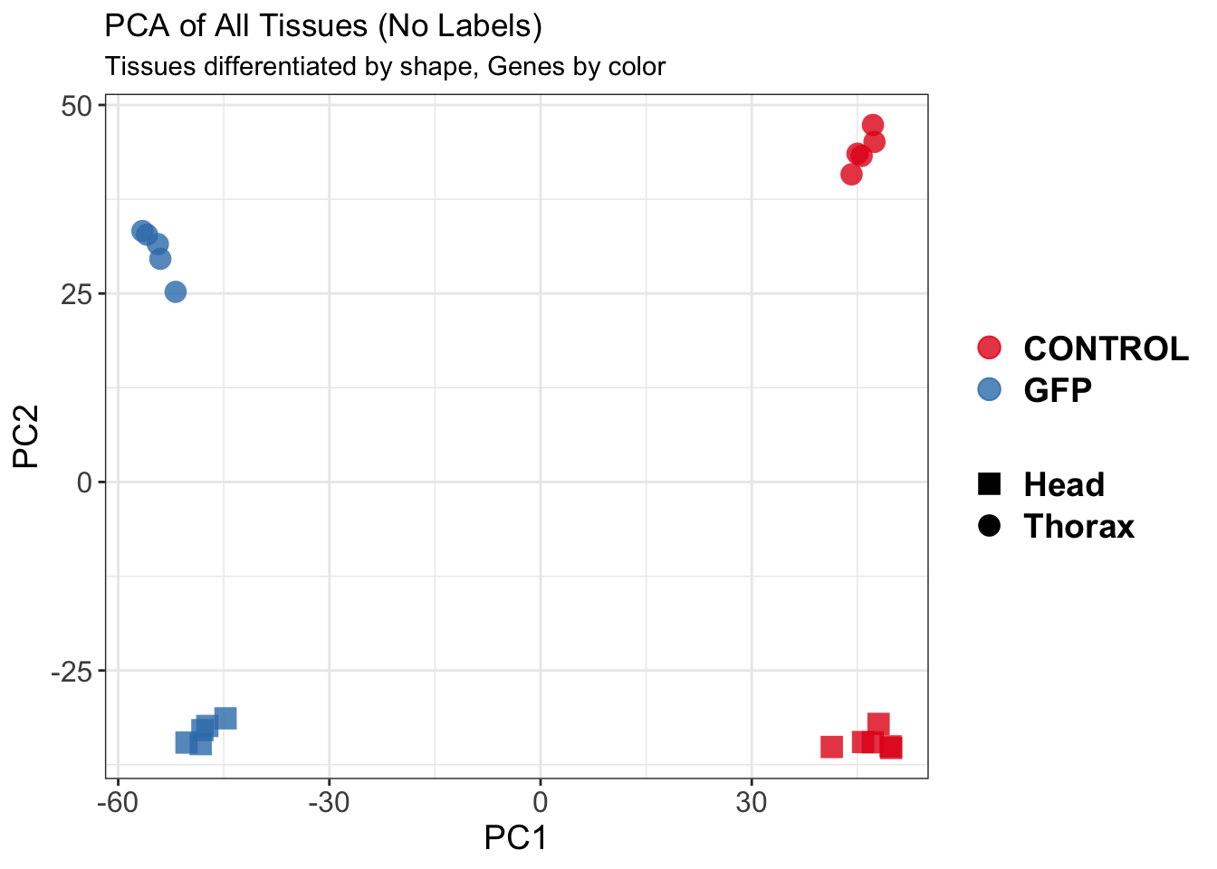
| Version | Author | Date |
|---|---|---|
| 9451c02 | Maeva TECHER | 2025-03-03 |
$WithLabel
| Version | Author | Date |
|---|---|---|
| 9451c02 | Maeva TECHER | 2025-03-03 |
The PCA plot shows clear distinction between tissue types, while gene silencing has a large variation within each tissue, and presents no distinct clear groupings for a single gene.
SVA
### SVA analysis to control for technical variation
dat <- counts(dds, normalized = TRUE)
idx <- rowMeans(dat) > 1
dat <- dat[idx, ]
mod <- model.matrix(~ Gene, colData(dds))
mod0 <- model.matrix(~ 1, colData(dds))
svseq <- svaseq(dat, mod, mod0)Number of significant surrogate variables is: 2
Iteration (out of 5 ):1 2 3 4 5 sva_plots <- create_sva_plots(svseq, dds, saveDir, intgroup = c("Tissue", "Gene"), max_sv = 4)
# Show stripcharts in the report
sva_plots$Stripcharts[[1]] # Show first stripchart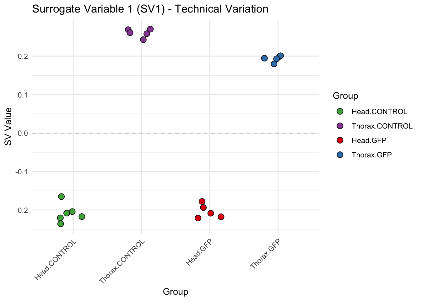
| Version | Author | Date |
|---|---|---|
| 9451c02 | Maeva TECHER | 2025-03-03 |
sva_plots$Stripcharts[[2]] # Show second stripchart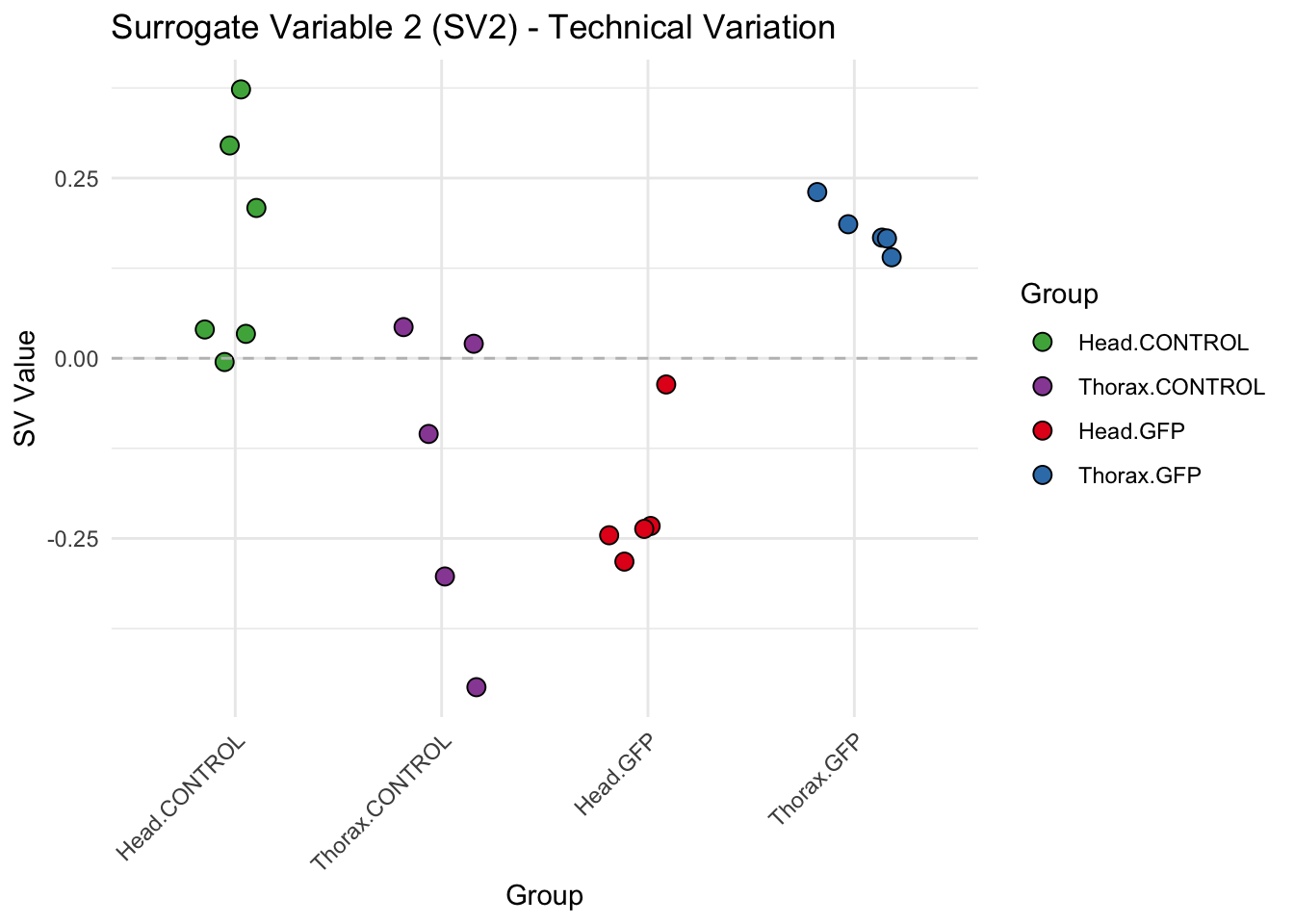
| Version | Author | Date |
|---|---|---|
| 9451c02 | Maeva TECHER | 2025-03-03 |
# Show scatter plots in the report
sva_plots$ScatterPlots[["1_2"]] # Show SV1 vs SV2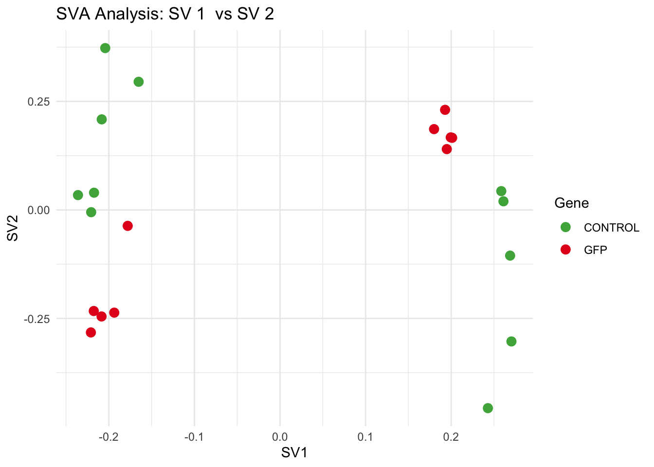
| Version | Author | Date |
|---|---|---|
| 9451c02 | Maeva TECHER | 2025-03-03 |
SV1 is clearly showing an effect of tissue. We rerun the
DESeq2 model but this time including the surrogate variable
SV2 and SV3 as a covariates only, as we know that the modeled variation
is more likely explained by tissue and gene variation rather than batch
effects.
ddssva <- dds
ddssva$SV1 <- svseq$sv[,1]
ddssva$SV2 <- svseq$sv[,2]
design(ddssva) <- ~ SV1 + SV2 + Gene
ddssva$Gene <- relevel(ddssva$Gene, ref = "CONTROL")
smallestGroupSize <- 5
keep <- rowSums(counts(ddssva) >= 10) >= smallestGroupSize
ddssva <- ddssva[keep,]
ddssva <- DESeq(ddssva)
ddssva <- ddssva[which(mcols(ddssva)$betaConv),] # remove non converging rows
### Extract results
message("Available contrasts are: ", paste(resultsNames(ddssva), collapse = ", "))
gfp <- results(ddssva, contrast = c("Gene", "GFP", "CONTROL"), alpha = 0.05)Volcano plots and Heatmaps
# Define contrast_sets
gfp_samples <- c("SGRE-HEAD-CRD-1","SGRE-HEAD-CRD-2","SGRE-HEAD-CRD-3","SGRE-HEAD-CRD-4","SGRE-HEAD-CRD-5",
"SGRE-HEAD-CRD-6","SggfpH1","SggfpH2","SggfpH3","SggfpH4","SggfpH5", "SGRE-THOX-CRD-1","SGRE-THOX-CRD-3","SGRE-THOX-CRD-4","SGRE-THOX-CRD-5",
"SGRE-THOX-CRD-6", "SggfpT1","SggfpT2","SggfpT3","SggfpT4","SggfpT5")
# Run full analysis
gfp_plots <- visualize_data_nopng(gfp, "GFP_vs_CONTROL", gfp_samples)
gfp_plots$volcano; gfp_plots$heatmap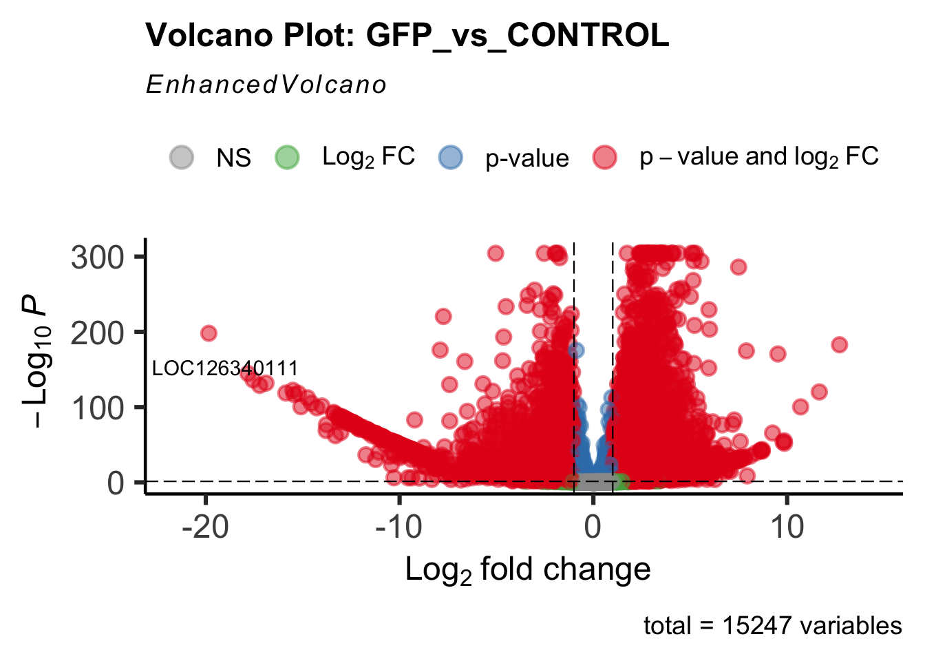
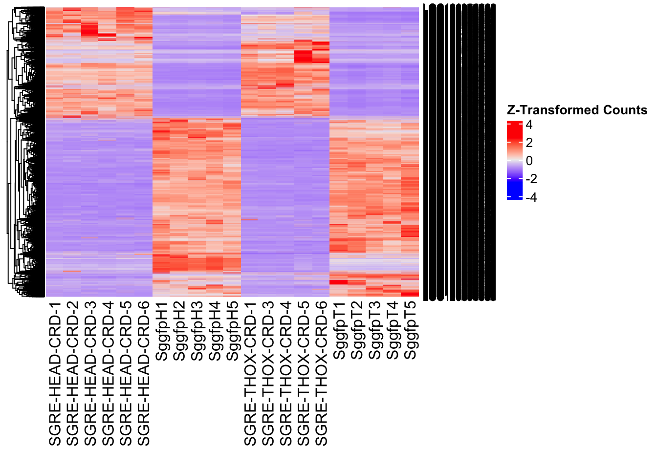
| Version | Author | Date |
|---|---|---|
| 9451c02 | Maeva TECHER | 2025-03-03 |
DEG tables
The following tables show the genes differentially expressed with at least an absolute log2fold change of > 1 considering all tissues together. Considering GFP as the reference state, upregulated genes in knockdown treatment in red and downregulated genes in knockdown treatment in blue. You can search for a gene of interest by writting a LOCID or description in the search bar or sort by column.
table_gfp <- generate_deg_table(ddssva, "Gene_GFP_vs_CONTROL", allspecies_df)
out of 15247 with nonzero total read count
adjusted p-value < 0.05
LFC > 0 (up) : 7769, 51%
LFC < 0 (down) : 5416, 36%
outliers [1] : 0, 0%
low counts [2] : 0, 0%
(mean count < 1)
[1] see 'cooksCutoff' argument of ?results
[2] see 'independentFiltering' argument of ?resultsTotal DEGs p-value < 0.05 and absolute logFoldChange > 1: 9396LFC > 1 (up) : 5833 (62.08%)LFC < -1 (down) : 3563 (37.92%)table_gfp$kable_tableSummary and Overlap
# Summarize DEGs for all contrasts
deg_summary <- bind_rows(
summarize_deg_counts(table_gfp, "GFP vs CONTROL")
)
# Display table using kable with styling
deg_summary %>%
kable("html", escape = FALSE, col.names = gsub("_", " ", names(.))) %>%
kable_styling("striped", full_width = TRUE) %>%
column_spec(2, color = "red", bold = TRUE) %>% # Upregulated in red
column_spec(3, color = "blue", bold = TRUE) %>% # Downregulated in blue
add_header_above(c("Summary of DEGs" = 3)) %>%
row_spec(0, bold = TRUE)| Contrast | Upregulated | Downregulated |
|---|---|---|
| GFP vs CONTROL | 5815 | 3553 |
# Define the list of RNAi contrasts
contrast_list <- c("GFP_vs_CONTROL")
# Initialize empty lists for storing Head-specific DEGs for each contrast
venn_data_up <- list()
venn_data_down <- list()
venn_data_all <- list()
# Function to load Head-specific DEGs for a given set of contrasts
load_deg_contrasts_head <- function(contrast_list) {
degs_up <- list()
degs_down <- list()
degs_all <- list()
for (contrast in contrast_list) {
deg_file <- file.path(workDir, "DEG_results/RNAi/All_GFP/", contrast, paste0("DEG_sigresults_", contrast, ".csv"))
if (!file.exists(deg_file)) {
message(paste("File missing for contrast:", contrast))
next # Skip if the file doesn't exist
}
deg_data <- read.csv(deg_file, stringsAsFactors = FALSE)
# Convert row names to a column if necessary
if ("X" %in% colnames(deg_data)) {
colnames(deg_data)[colnames(deg_data) == "X"] <- "GeneID"
}
# Check if data is empty
if (nrow(deg_data) == 0) {
message(paste("No data for contrast:", contrast))
next
}
# Select significant DEGs (Up, Down, All)
degs_up[[contrast]] <- deg_data %>%
filter(padj < 0.05 & log2FoldChange >= 1) %>%
pull(GeneID) # Extract GeneID column
degs_down[[contrast]] <- deg_data %>%
filter(padj < 0.05 & log2FoldChange <= -1) %>%
pull(GeneID) # Extract GeneID column
degs_all[[contrast]] <- deg_data %>%
filter(padj < 0.05 & abs(log2FoldChange) >= 1) %>%
pull(GeneID) # Extract GeneID column
}
return(list(up = degs_up, down = degs_down, all = degs_all))
}
# Load DEG data for the defined contrasts (Head tissue only)
venn_data_contrasts <- load_deg_contrasts_head(contrast_list)
# Prepare the data for the Venn diagrams
venn_data_up <- venn_data_contrasts$up
venn_data_down <- venn_data_contrasts$down
venn_data_all <- venn_data_contrasts$allHead tissue
saveDir <- paste0(workDir,"/DEG_results/RNAi/Head_GFP")
dir.create(saveDir)
### Prepare Sample CSV file #####
samples <- read.delim(file.path(workDir, "list/RNAi/Head_RNAi_GFPCRDsample_list.csv"), sep = ",", row.names = 1, header = TRUE)
files <- file.path(workDir, "readcounts/RNAi/", samples$Tissue, samples$Filename)
names(files) <- row.names(samples)
if (all(file.exists(files))) {
message("All the files exist!")
} else {
warning("Some files are missing!")
}All the files exist!### **Standardized Count Matrix Creation**
# Extract all gene lists first
gene_lists <- map(files, function(sample) {
fread(sample, sep = "\t", header = FALSE)[, 1] # Extract Gene IDs (column 1)
})
# Get a unique set of all gene IDs across all samples
all_genes <- unique(unlist(gene_lists))
# Create a named list to store count data with standardized rows
cts_list <- map(files, function(sample) {
data_count <- fread(sample, sep = "\t", header = FALSE)
col_name <- gsub("_counts.txt", "", basename(sample)) # Clean sample name
# Convert to data frame with correct column names
data_count <- setNames(data.frame(data_count[, 1:2]), c("GeneID", col_name))
# Ensure all gene IDs are present (fill missing values with 0)
data_count <- full_join(data.frame(GeneID = all_genes), data_count, by = "GeneID") %>%
mutate(across(where(is.numeric), ~ replace_na(., 0))) # Fill NA with 0
return(data_count)
})
# Merge all samples based on GeneID
cts <- reduce(cts_list, full_join, by = "GeneID")
# Convert to matrix for DESeq2
cts_matrix <- as.matrix(cts[, -1]) # Remove GeneID column for count matrix
rownames(cts_matrix) <- cts$GeneID # Set GeneID as rownames
rm(cts_list) # Free memoryWhile for bulk RNAseq on head and thorax for all species, the DEGs model was made between isolated and crowded individuals (with isolated as the reference state), here, the DEG analysis will be carried between GFP knock-down nymphs (as reference state) vs Hexamerins / Juvenile Hormones / Inositol / Uncharacterized proteins.
### Build DESeq2 Object
dds <- DESeqDataSetFromMatrix(countData = cts_matrix,
colData = samples,
design = ~ Gene)
dds$Gene <- relevel(dds$Gene, ref = "CONTROL")
smallestGroupSize <- 5
keep <- rowSums(counts(dds) >= 10) >= smallestGroupSize
dds <- dds[keep,]
dds <- DESeq(dds)Normalization and PCA
# Plot PCA and investigate quality metrics
vsd <- vst(dds, blind = TRUE)
# Perform PCA
pca_data <- plotPCA(vsd, intgroup = c("Tissue", "Gene"), returnData = TRUE)
# Define colors for genes (slightly transparent) and shapes for tissues
gene_colors <- scale_color_manual(values = alpha(brewer.pal(n = length(unique(pca_data$Gene)), name = "Set1"), 0.8)) # Points are transparent
tissue_shapes <- scale_shape_manual(values = seq(15, 15 + length(unique(pca_data$Tissue))))
# **PCA without labels**
p_pca_nolabel <- ggplot(pca_data, aes(x = PC1, y = PC2, color = Gene, shape = Tissue)) +
geom_point(size = 4) +
gene_colors +
tissue_shapes +
theme_bw() +
theme(legend.title = element_blank(),
legend.text = element_text(face = "bold", size = 14),
axis.text = element_text(size = 12),
axis.title = element_text(size = 14)) +
ggtitle("PCA of All Tissues (No Labels)", subtitle = "Tissues differentiated by shape, Genes by color")
# Save PCA without labels
ggsave(paste0(saveDir, "/PCA_Tissue_Gene_NoLabel.png"), plot = p_pca_nolabel, width = 10, height = 10, dpi = 600, device = "png")
# **PCA with labels**
p_pca_label <- ggplot(pca_data, aes(x = PC1, y = PC2, color = Gene, shape = Tissue)) +
geom_point(size = 4) +
geom_text_repel(aes(label = name), size = 4, color = "black", max.overlaps = 20) + # Labels are fully visible
gene_colors +
tissue_shapes +
theme_bw() +
theme(legend.title = element_blank(),
legend.text = element_text(face = "bold", size = 14),
axis.text = element_text(size = 12),
axis.title = element_text(size = 14)) +
ggtitle("PCA of All Tissues (With Labels)", subtitle = "Tissues differentiated by shape, Genes by color")
# Save PCA with labels
ggsave(paste0(saveDir, "/PCA_Tissue_Gene_Label.png"), plot = p_pca_label, width = 10, height = 10, dpi = 600, device = "png")
# **Return plots for knitr/RMarkdown**
list(NoLabel = p_pca_nolabel, WithLabel = p_pca_label)$NoLabel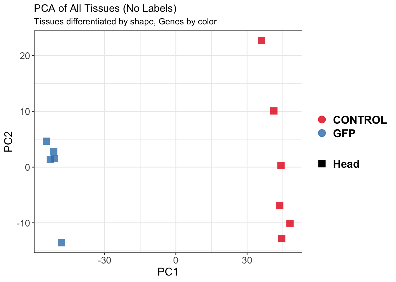
| Version | Author | Date |
|---|---|---|
| 9451c02 | Maeva TECHER | 2025-03-03 |
$WithLabel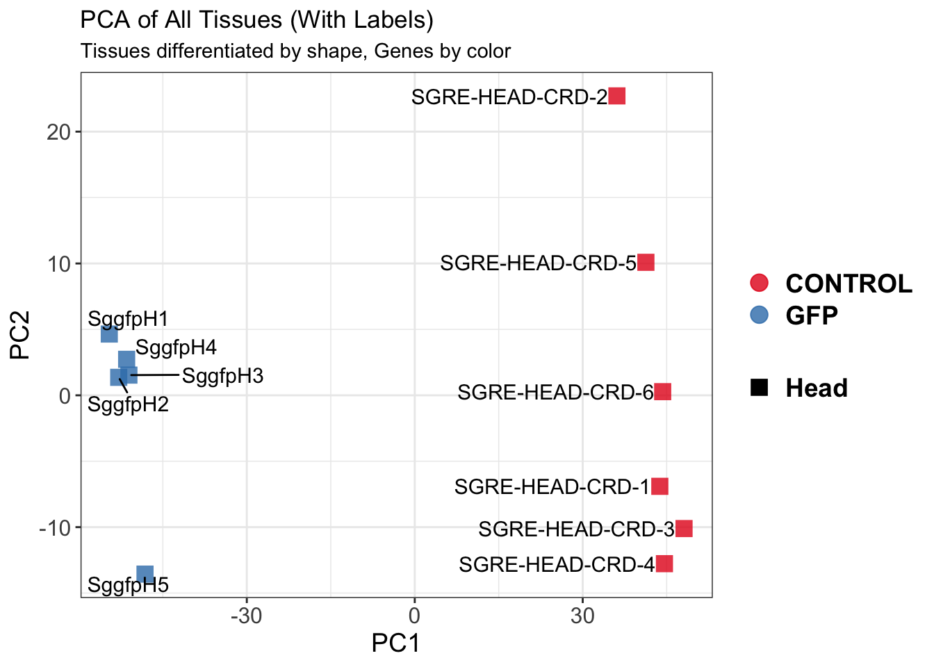
| Version | Author | Date |
|---|---|---|
| 9451c02 | Maeva TECHER | 2025-03-03 |
The PCA plot shows clear distinction between tissue types, while gene silencing has a large variation within each tissue, and presents no distinct clear groupings for a single gene.
SVA
### SVA analysis to control for technical variation
dat <- counts(dds, normalized = TRUE)
idx <- rowMeans(dat) > 1
dat <- dat[idx, ]
mod <- model.matrix(~ Gene, colData(dds))
mod0 <- model.matrix(~ 1, colData(dds))
svseq <- svaseq(dat, mod, mod0)Number of significant surrogate variables is: 4
Iteration (out of 5 ):1 2 3 4 5 sva_plots <- create_sva_plots(svseq, dds, saveDir, intgroup = c("Tissue", "Gene"), max_sv = 7)
# Show stripcharts in the report
sva_plots$Stripcharts[[1]] # Show first stripchart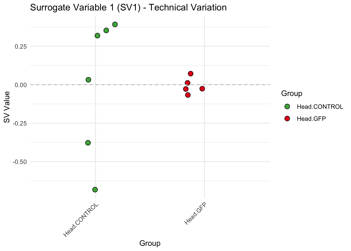
| Version | Author | Date |
|---|---|---|
| 9451c02 | Maeva TECHER | 2025-03-03 |
sva_plots$Stripcharts[[2]] # Show second stripchart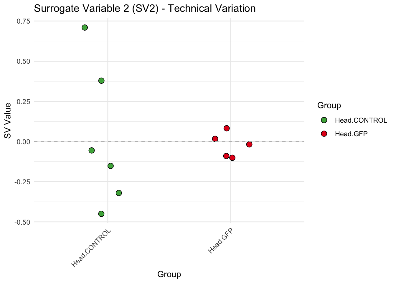
| Version | Author | Date |
|---|---|---|
| 9451c02 | Maeva TECHER | 2025-03-03 |
sva_plots$Stripcharts[[3]] # Show third stripchart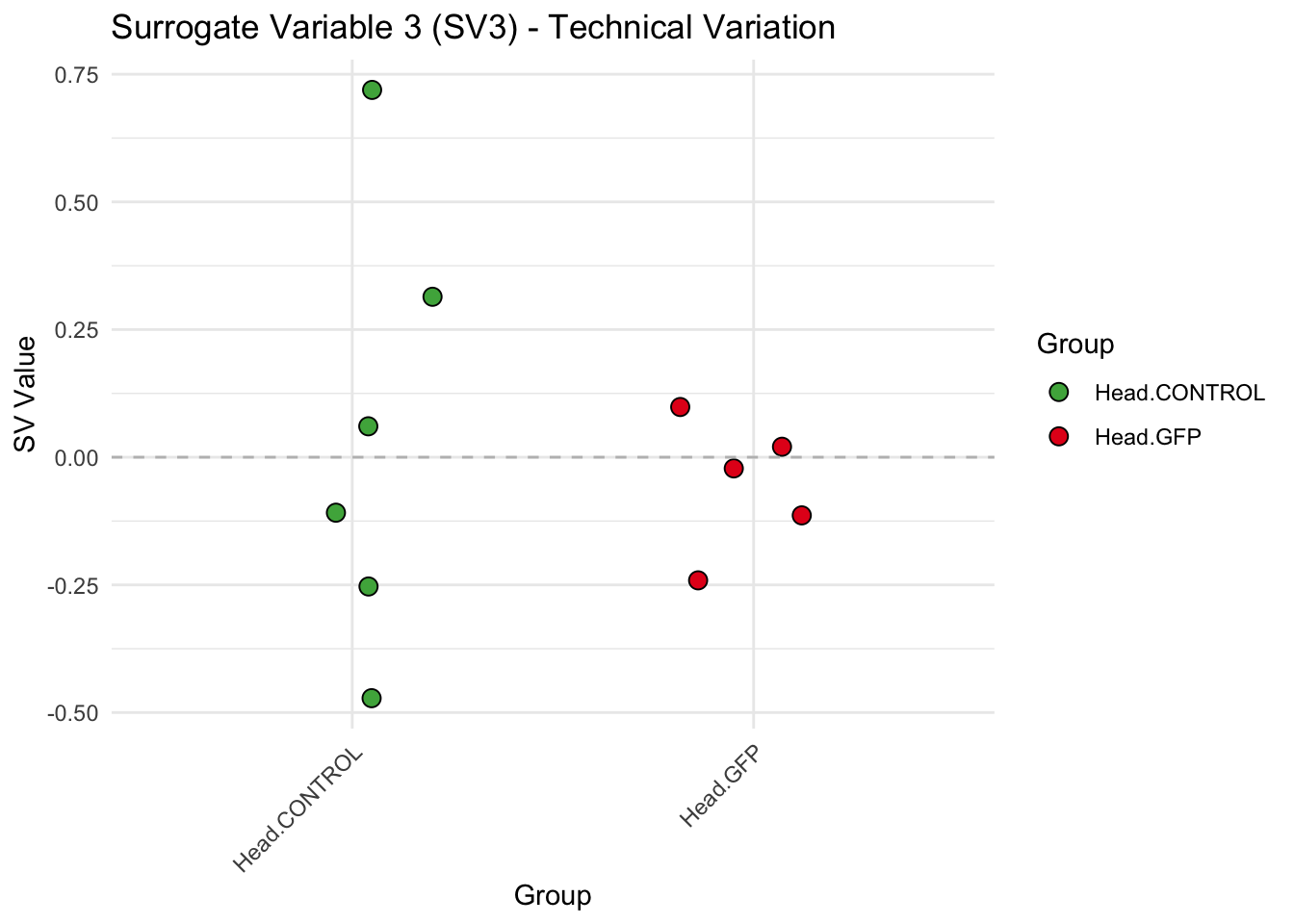
| Version | Author | Date |
|---|---|---|
| 9451c02 | Maeva TECHER | 2025-03-03 |
sva_plots$Stripcharts[[4]] 
| Version | Author | Date |
|---|---|---|
| 9451c02 | Maeva TECHER | 2025-03-03 |
# Show scatter plots in the report
sva_plots$ScatterPlots[["1_2"]] # Show SV1 vs SV2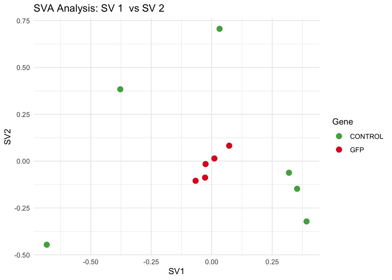
| Version | Author | Date |
|---|---|---|
| 9451c02 | Maeva TECHER | 2025-03-03 |
sva_plots$ScatterPlots[["1_3"]] # Show SV1 vs SV3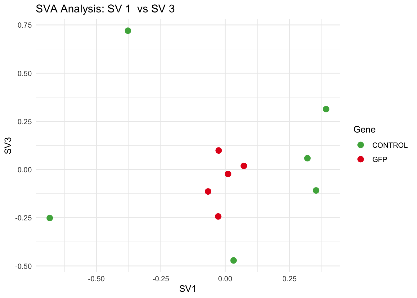
| Version | Author | Date |
|---|---|---|
| 9451c02 | Maeva TECHER | 2025-03-03 |
sva_plots$ScatterPlots[["2_3"]] # Show SV2 vs SV3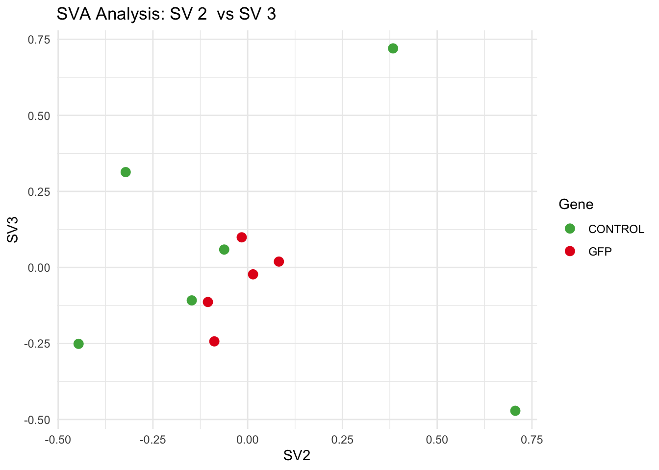
| Version | Author | Date |
|---|---|---|
| 9451c02 | Maeva TECHER | 2025-03-03 |
SV1 is clearly showing an effect of tissue. We rerun the
DESeq2 model but this time including the surrogate variable
SV2 and SV3 as a covariates only, as we know that the modeled variation
is more likely explained by tissue and gene variation rather than batch
effects.
ddssva <- dds
ddssva$SV1 <- svseq$sv[,1]
ddssva$SV2 <- svseq$sv[,2]
ddssva$SV3 <- svseq$sv[,3]
ddssva$SV4 <- svseq$sv[,4]
design(ddssva) <- ~ SV1 + SV2 + SV3 + SV4 + Gene
ddssva$Gene <- relevel(ddssva$Gene, ref = "CONTROL")
smallestGroupSize <- 5
keep <- rowSums(counts(ddssva) >= 10) >= smallestGroupSize
ddssva <- ddssva[keep,]
ddssva <- DESeq(ddssva)
ddssva <- ddssva[which(mcols(ddssva)$betaConv),] # remove non converging rows
### Extract results
message("Available contrasts are: ", paste(resultsNames(ddssva), collapse = ", "))
gfp <- results(ddssva, contrast = c("Gene", "GFP", "CONTROL"), alpha = 0.05)Volcano plots and Heatmaps
# Define contrast_sets
gfp_samples <- c("SGRE-HEAD-CRD-1","SGRE-HEAD-CRD-2","SGRE-HEAD-CRD-3","SGRE-HEAD-CRD-4","SGRE-HEAD-CRD-5",
"SGRE-HEAD-CRD-6","SggfpH1","SggfpH2","SggfpH3","SggfpH4","SggfpH5")
# Run full analysis
gfp_plots <- visualize_data_nopng(gfp, "GFP_vs_CONTROL", gfp_samples)
gfp_plots$volcano; gfp_plots$heatmap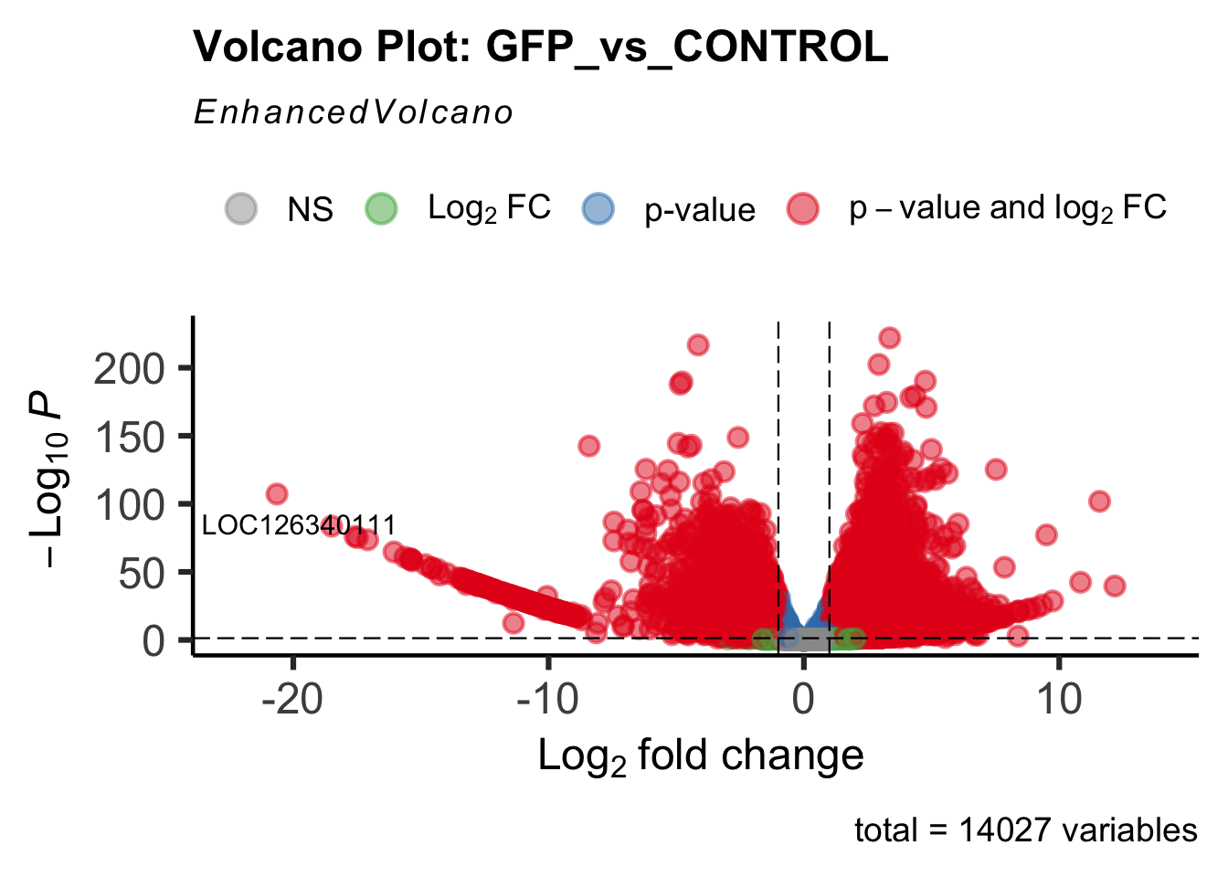
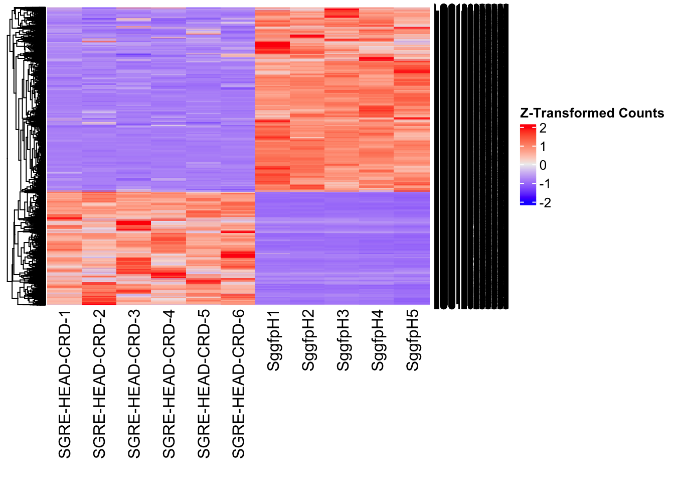
| Version | Author | Date |
|---|---|---|
| 9451c02 | Maeva TECHER | 2025-03-03 |
DEG tables
The following tables show the genes differentially expressed with at least an absolute log2fold change of > 1 considering Head tissues only. Considering GFP as the reference state, upregulated genes in knockdown treatment in red and downregulated genes in knockdown treatment in blue. You can search for a gene of interest by writting a LOCID or description in the search bar or sort by column.
# Generate tables for each contrast
table_gfp <- generate_deg_table(ddssva, "Gene_GFP_vs_CONTROL", allspecies_df)
out of 14027 with nonzero total read count
adjusted p-value < 0.05
LFC > 0 (up) : 6503, 46%
LFC < 0 (down) : 4639, 33%
outliers [1] : 0, 0%
low counts [2] : 0, 0%
(mean count < 2)
[1] see 'cooksCutoff' argument of ?results
[2] see 'independentFiltering' argument of ?resultsTotal DEGs p-value < 0.05 and absolute logFoldChange > 1: 8238LFC > 1 (up) : 5092 (61.81%)LFC < -1 (down) : 3146 (38.19%)table_gfp$kable_tableSummary and Overlap
# Summarize DEGs for all contrasts
deg_summary <- bind_rows(
summarize_deg_counts(table_gfp, "GFP vs CONTROL")
)
# Display table using kable with styling
deg_summary %>%
kable("html", escape = FALSE, col.names = gsub("_", " ", names(.))) %>%
kable_styling("striped", full_width = TRUE) %>%
column_spec(2, color = "red", bold = TRUE) %>% # Upregulated in red
column_spec(3, color = "blue", bold = TRUE) %>% # Downregulated in blue
add_header_above(c("Summary of DEGs" = 3)) %>%
row_spec(0, bold = TRUE)| Contrast | Upregulated | Downregulated |
|---|---|---|
| GFP vs CONTROL | 5068 | 3130 |
# Define the list of RNAi contrasts
contrast_list <- c("GFP_vs_CONTROL")
# Initialize empty lists for storing Head-specific DEGs for each contrast
venn_data_up <- list()
venn_data_down <- list()
venn_data_all <- list()
# Function to load Head-specific DEGs for a given set of contrasts
load_deg_contrasts_head <- function(contrast_list) {
degs_up <- list()
degs_down <- list()
degs_all <- list()
for (contrast in contrast_list) {
deg_file <- file.path(workDir, "DEG_results/RNAi/Head_GFP/", contrast, paste0("DEG_sigresults_", contrast, ".csv"))
if (!file.exists(deg_file)) {
message(paste("File missing for contrast:", contrast))
next # Skip if the file doesn't exist
}
deg_data <- read.csv(deg_file, stringsAsFactors = FALSE)
# Convert row names to a column if necessary
if ("X" %in% colnames(deg_data)) {
colnames(deg_data)[colnames(deg_data) == "X"] <- "GeneID"
}
# Check if data is empty
if (nrow(deg_data) == 0) {
message(paste("No data for contrast:", contrast))
next
}
# Select significant DEGs (Up, Down, All)
degs_up[[contrast]] <- deg_data %>%
filter(padj < 0.05 & log2FoldChange >= 1) %>%
pull(GeneID) # Extract GeneID column
degs_down[[contrast]] <- deg_data %>%
filter(padj < 0.05 & log2FoldChange <= -1) %>%
pull(GeneID) # Extract GeneID column
degs_all[[contrast]] <- deg_data %>%
filter(padj < 0.05 & abs(log2FoldChange) >= 1) %>%
pull(GeneID) # Extract GeneID column
}
return(list(up = degs_up, down = degs_down, all = degs_all))
}
# Load DEG data for the defined contrasts (Head tissue only)
venn_data_contrasts <- load_deg_contrasts_head(contrast_list)
# Prepare the data for the Venn diagrams
venn_data_up <- venn_data_contrasts$up
venn_data_down <- venn_data_contrasts$down
venn_data_all <- venn_data_contrasts$allThorax tissue
saveDir <- paste0(workDir,"/DEG_results/RNAi/Thorax_GFP")
dir.create(saveDir)
### Prepare Sample CSV file #####
samples <- read.delim(file.path(workDir, "list/RNAi/Thorax_RNAi_GFPCRDsample_list.csv"), sep = ",", row.names = 1, header = TRUE)
files <- file.path(workDir, "readcounts/RNAi/", samples$Tissue, samples$Filename)
names(files) <- row.names(samples)
if (all(file.exists(files))) {
message("All the files exist!")
} else {
warning("Some files are missing!")
}All the files exist!### **Standardized Count Matrix Creation**
# Extract all gene lists first
gene_lists <- map(files, function(sample) {
fread(sample, sep = "\t", header = FALSE)[, 1] # Extract Gene IDs (column 1)
})
# Get a unique set of all gene IDs across all samples
all_genes <- unique(unlist(gene_lists))
# Create a named list to store count data with standardized rows
cts_list <- map(files, function(sample) {
data_count <- fread(sample, sep = "\t", header = FALSE)
col_name <- gsub("_counts.txt", "", basename(sample)) # Clean sample name
# Convert to data frame with correct column names
data_count <- setNames(data.frame(data_count[, 1:2]), c("GeneID", col_name))
# Ensure all gene IDs are present (fill missing values with 0)
data_count <- full_join(data.frame(GeneID = all_genes), data_count, by = "GeneID") %>%
mutate(across(where(is.numeric), ~ replace_na(., 0))) # Fill NA with 0
return(data_count)
})
# Merge all samples based on GeneID
cts <- reduce(cts_list, full_join, by = "GeneID")
# Convert to matrix for DESeq2
cts_matrix <- as.matrix(cts[, -1]) # Remove GeneID column for count matrix
rownames(cts_matrix) <- cts$GeneID # Set GeneID as rownames
rm(cts_list) # Free memoryWhile for bulk RNAseq on head and thorax for all species, the DEGs model was made between isolated and crowded individuals (with isolated as the reference state), here, the DEG analysis will be carried between GFP knock-down nymphs (as reference state) vs Hexamerins / Juvenile Hormones / Inositol / Uncharacterized proteins.
### Build DESeq2 Object
dds <- DESeqDataSetFromMatrix(countData = cts_matrix,
colData = samples,
design = ~ Gene)
dds$Gene <- relevel(dds$Gene, ref = "CONTROL")
smallestGroupSize <- 5
keep <- rowSums(counts(dds) >= 10) >= smallestGroupSize
dds <- dds[keep,]
dds <- DESeq(dds)Normalization and PCA
# Plot PCA and investigate quality metrics
vsd <- vst(dds, blind = TRUE)
# Perform PCA
pca_data <- plotPCA(vsd, intgroup = c("Tissue", "Gene"), returnData = TRUE)
# Define colors for genes (slightly transparent) and shapes for tissues
gene_colors <- scale_color_manual(values = alpha(brewer.pal(n = length(unique(pca_data$Gene)), name = "Set1"), 0.8)) # Points are transparent
tissue_shapes <- scale_shape_manual(values = seq(15, 15 + length(unique(pca_data$Tissue))))
# **PCA without labels**
p_pca_nolabel <- ggplot(pca_data, aes(x = PC1, y = PC2, color = Gene, shape = Tissue)) +
geom_point(size = 4) +
gene_colors +
tissue_shapes +
theme_bw() +
theme(legend.title = element_blank(),
legend.text = element_text(face = "bold", size = 14),
axis.text = element_text(size = 12),
axis.title = element_text(size = 14)) +
ggtitle("PCA of All Tissues (No Labels)", subtitle = "Tissues differentiated by shape, Genes by color")
# Save PCA without labels
ggsave(paste0(saveDir, "/PCA_Tissue_Gene_NoLabel.png"), plot = p_pca_nolabel, width = 10, height = 10, dpi = 600, device = "png")
# **PCA with labels**
p_pca_label <- ggplot(pca_data, aes(x = PC1, y = PC2, color = Gene, shape = Tissue)) +
geom_point(size = 4) +
geom_text_repel(aes(label = name), size = 4, color = "black", max.overlaps = 20) + # Labels are fully visible
gene_colors +
tissue_shapes +
theme_bw() +
theme(legend.title = element_blank(),
legend.text = element_text(face = "bold", size = 14),
axis.text = element_text(size = 12),
axis.title = element_text(size = 14)) +
ggtitle("PCA of All Tissues (With Labels)", subtitle = "Tissues differentiated by shape, Genes by color")
# Save PCA with labels
ggsave(paste0(saveDir, "/PCA_Tissue_Gene_Label.png"), plot = p_pca_label, width = 10, height = 10, dpi = 600, device = "png")
# **Return plots for knitr/RMarkdown**
list(NoLabel = p_pca_nolabel, WithLabel = p_pca_label)$NoLabel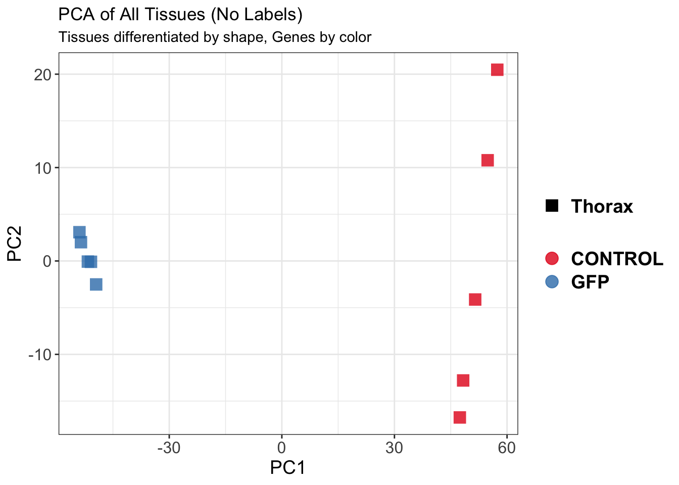
| Version | Author | Date |
|---|---|---|
| 9451c02 | Maeva TECHER | 2025-03-03 |
$WithLabel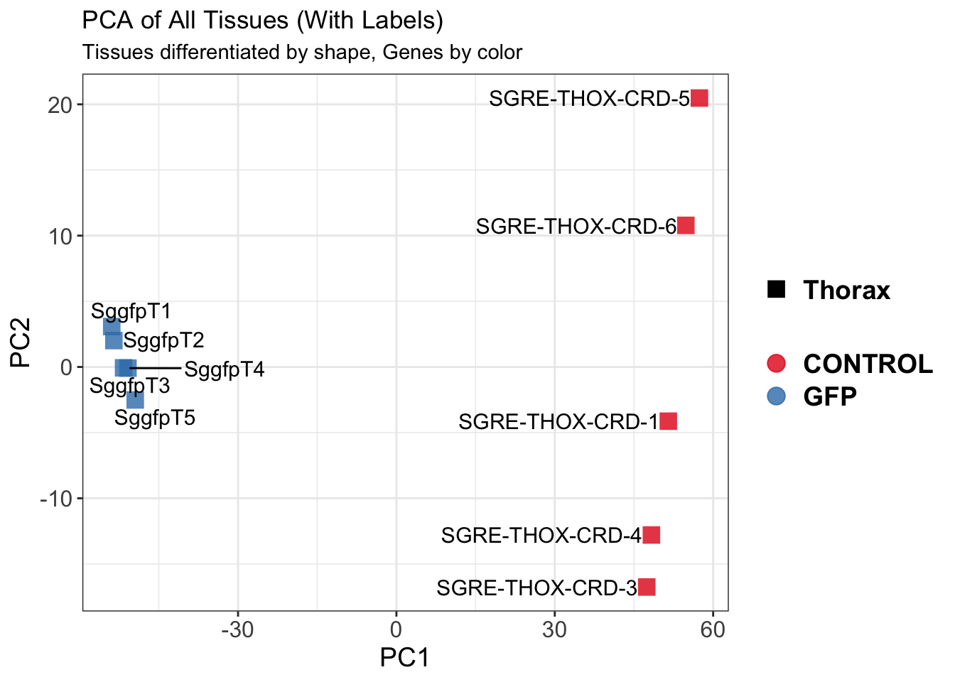
| Version | Author | Date |
|---|---|---|
| 9451c02 | Maeva TECHER | 2025-03-03 |
The PCA plot shows clear distinction between tissue types, while gene silencing has a large variation within each tissue, and presents no distinct clear groupings for a single gene.
SVA
### SVA analysis to control for technical variation
dat <- counts(dds, normalized = TRUE)
idx <- rowMeans(dat) > 1
dat <- dat[idx, ]
mod <- model.matrix(~ Gene, colData(dds))
mod0 <- model.matrix(~ 1, colData(dds))
svseq <- svaseq(dat, mod, mod0)Number of significant surrogate variables is: 2
Iteration (out of 5 ):1 2 3 4 5 sva_plots <- create_sva_plots(svseq, dds, saveDir, intgroup = c("Tissue", "Gene"), max_sv = 6)
# Show stripcharts in the report
sva_plots$Stripcharts[[1]] # Show first stripchart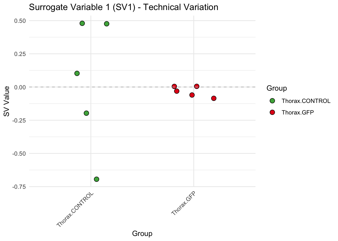
| Version | Author | Date |
|---|---|---|
| 9451c02 | Maeva TECHER | 2025-03-03 |
sva_plots$Stripcharts[[2]] # Show second stripchart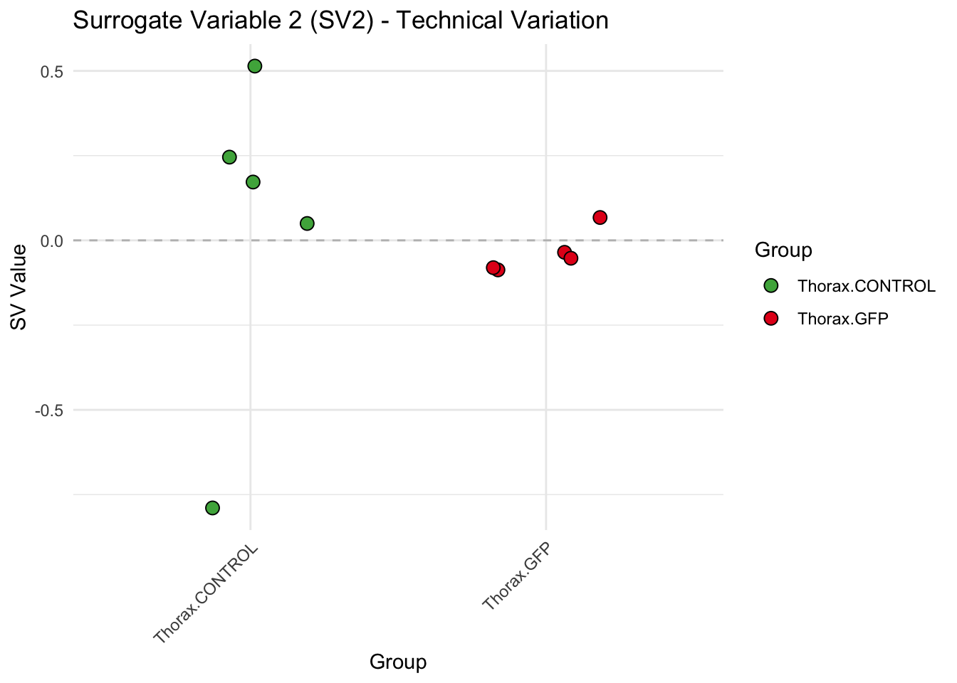
| Version | Author | Date |
|---|---|---|
| 9451c02 | Maeva TECHER | 2025-03-03 |
# Show scatter plots in the report
sva_plots$ScatterPlots[["1_2"]] # Show SV1 vs SV2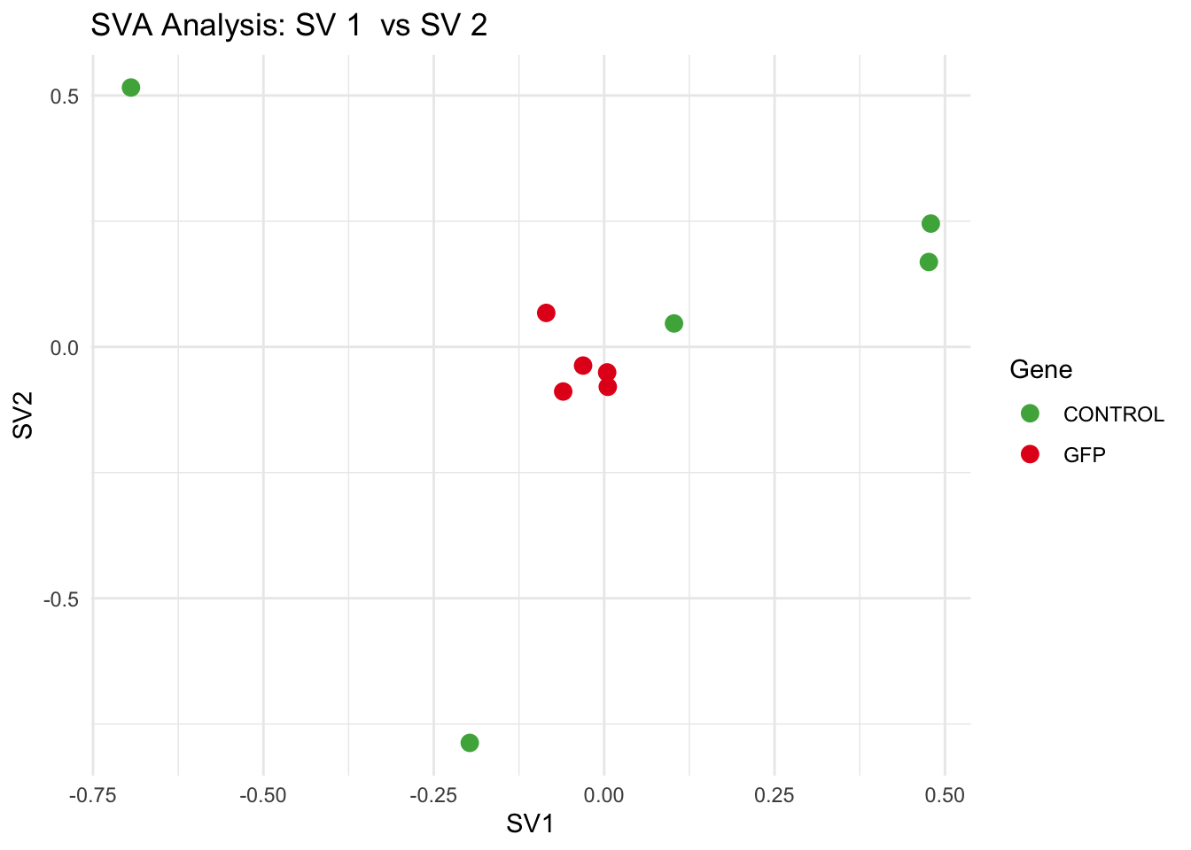
| Version | Author | Date |
|---|---|---|
| 9451c02 | Maeva TECHER | 2025-03-03 |
SV1 is clearly showing an effect of tissue. We rerun the
DESeq2 model but this time including the surrogate variable
SV2 and SV3 as a covariates only, as we know that the modeled variation
is more likely explained by tissue and gene variation rather than batch
effects.
ddssva <- dds
ddssva$SV1 <- svseq$sv[,1]
ddssva$SV2 <- svseq$sv[,2]
design(ddssva) <- ~ SV1 + SV2 + Gene
ddssva$Gene <- relevel(ddssva$Gene, ref = "CONTROL")
smallestGroupSize <- 5
keep <- rowSums(counts(ddssva) >= 10) >= smallestGroupSize
ddssva <- ddssva[keep,]
ddssva <- DESeq(ddssva)
ddssva <- ddssva[which(mcols(ddssva)$betaConv),] # remove non converging rows
### Extract results
message("Available contrasts are: ", paste(resultsNames(ddssva), collapse = ", "))
gfp <- results(ddssva, contrast = c("Gene", "GFP", "CONTROL"), alpha = 0.05)Volcano plots and Heatmaps
# Define contrast_sets
gfp_samples <- c("SGRE-THOX-CRD-1","SGRE-THOX-CRD-3","SGRE-THOX-CRD-4","SGRE-THOX-CRD-5",
"SGRE-THOX-CRD-6", "SggfpT1","SggfpT2","SggfpT3","SggfpT4","SggfpT5")
# Run full analysis
gfp_plots <- visualize_data_nopng(gfp, "GFP_vs_CONTROL", gfp_samples)
gfp_plots$volcano; gfp_plots$heatmap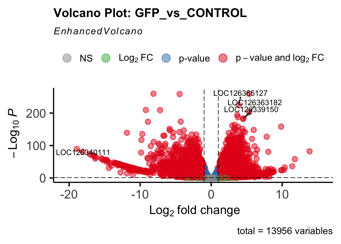
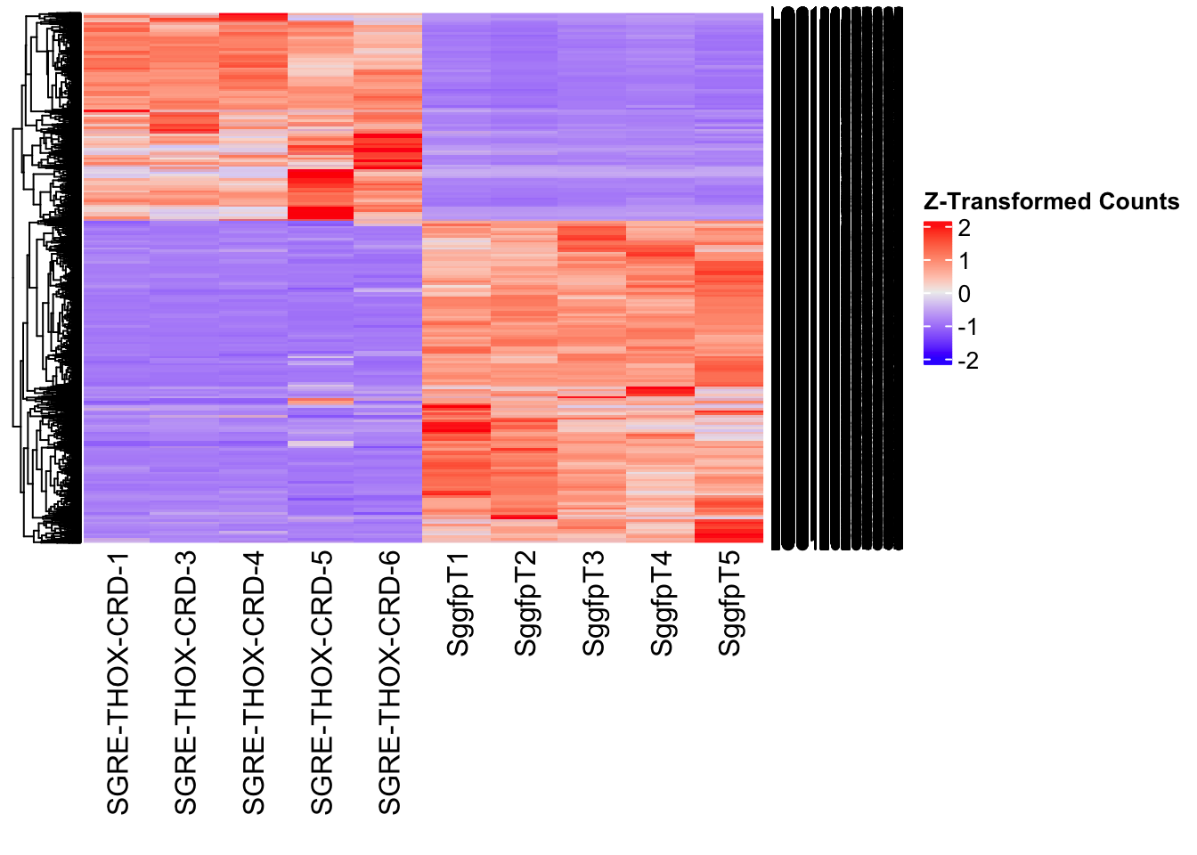
| Version | Author | Date |
|---|---|---|
| 9451c02 | Maeva TECHER | 2025-03-03 |
DEG tables
The following tables show the genes differentially expressed with at least an absolute log2fold change of > 1 considering Head tissues only. Considering GFP as the reference state, upregulated genes in knockdown treatment in red and downregulated genes in knockdown treatment in blue. You can search for a gene of interest by writting a LOCID or description in the search bar or sort by column.
# Generate tables for each contrast
table_gfp <- generate_deg_table(ddssva, "Gene_GFP_vs_CONTROL", allspecies_df)
out of 13956 with nonzero total read count
adjusted p-value < 0.05
LFC > 0 (up) : 6533, 47%
LFC < 0 (down) : 4691, 34%
outliers [1] : 0, 0%
low counts [2] : 0, 0%
(mean count < 2)
[1] see 'cooksCutoff' argument of ?results
[2] see 'independentFiltering' argument of ?resultsTotal DEGs p-value < 0.05 and absolute logFoldChange > 1: 8593LFC > 1 (up) : 5229 (60.85%)LFC < -1 (down) : 3364 (39.15%)table_gfp$kable_tableSummary and Overlap
# Summarize DEGs for all contrasts
deg_summary <- bind_rows(
summarize_deg_counts(table_gfp, "GFP vs CONTROL")
)
# Display table using kable with styling
deg_summary %>%
kable("html", escape = FALSE, col.names = gsub("_", " ", names(.))) %>%
kable_styling("striped", full_width = TRUE) %>%
column_spec(2, color = "red", bold = TRUE) %>% # Upregulated in red
column_spec(3, color = "blue", bold = TRUE) %>% # Downregulated in blue
add_header_above(c("Summary of DEGs" = 3)) %>%
row_spec(0, bold = TRUE)| Contrast | Upregulated | Downregulated |
|---|---|---|
| GFP vs CONTROL | 5196 | 3353 |
# Define the list of RNAi contrasts
contrast_list <- c("GFP_vs_CONTROL")
# Initialize empty lists for storing Head-specific DEGs for each contrast
venn_data_up <- list()
venn_data_down <- list()
venn_data_all <- list()
# Function to load Head-specific DEGs for a given set of contrasts
load_deg_contrasts_head <- function(contrast_list) {
degs_up <- list()
degs_down <- list()
degs_all <- list()
for (contrast in contrast_list) {
deg_file <- file.path(workDir, "DEG_results/RNAi/Thorax_GFP/", contrast, paste0("DEG_sigresults_", contrast, ".csv"))
if (!file.exists(deg_file)) {
message(paste("File missing for contrast:", contrast))
next # Skip if the file doesn't exist
}
deg_data <- read.csv(deg_file, stringsAsFactors = FALSE)
# Convert row names to a column if necessary
if ("X" %in% colnames(deg_data)) {
colnames(deg_data)[colnames(deg_data) == "X"] <- "GeneID"
}
# Check if data is empty
if (nrow(deg_data) == 0) {
message(paste("No data for contrast:", contrast))
next
}
# Select significant DEGs (Up, Down, All)
degs_up[[contrast]] <- deg_data %>%
filter(padj < 0.05 & log2FoldChange >= 1) %>%
pull(GeneID) # Extract GeneID column
degs_down[[contrast]] <- deg_data %>%
filter(padj < 0.05 & log2FoldChange <= -1) %>%
pull(GeneID) # Extract GeneID column
degs_all[[contrast]] <- deg_data %>%
filter(padj < 0.05 & abs(log2FoldChange) >= 1) %>%
pull(GeneID) # Extract GeneID column
}
return(list(up = degs_up, down = degs_down, all = degs_all))
}
# Load DEG data for the defined contrasts (Head tissue only)
venn_data_contrasts <- load_deg_contrasts_head(contrast_list)
# Prepare the data for the Venn diagrams
venn_data_up <- venn_data_contrasts$up
venn_data_down <- venn_data_contrasts$down
venn_data_all <- venn_data_contrasts$allExcluding rRNA
All tissue together
Minor changes here are made compared to the DESeq2
results regarding the importation of samples to transform into a
matrix.
Sample names are structured as follow: {Sg}{gene}{#} {Sg} = Schistocerca gregaria {gene} = gene abbreviation gfp, hex1, hex2, jhmt, miox and unch H/T{#} = biological replicate
saveDir <- paste0(workDir,"/DEG_results/RNAi/All_GFP_no_rRNA")
dir.create(saveDir)
### Prepare Sample CSV file #####
samples <- read.delim(file.path(workDir, "list/RNAi/All_RNAi_GFPCRDsample_list.csv"), sep = ",", row.names = 1, header = TRUE)
files <- file.path(workDir, "readcounts/RNAi/", samples$Tissue, samples$Filename)
names(files) <- row.names(samples)
if (all(file.exists(files))) {
message("All the files exist!")
} else {
warning("Some files are missing!")
}All the files exist!### **Standardized Count Matrix Creation**
# Extract all gene lists first
gene_lists <- map(files, function(sample) {
fread(sample, sep = "\t", header = FALSE)[, 1] # Extract Gene IDs (column 1)
})
# Get a unique set of all gene IDs across all samples
all_genes <- unique(unlist(gene_lists))
# Create a named list to store count data with standardized rows
cts_list <- map(files, function(sample) {
data_count <- fread(sample, sep = "\t", header = FALSE)
col_name <- gsub("_counts.txt", "", basename(sample)) # Clean sample name
# Convert to data frame with correct column names
data_count <- setNames(data.frame(data_count[, 1:2]), c("GeneID", col_name))
# Ensure all gene IDs are present (fill missing values with 0)
data_count <- full_join(data.frame(GeneID = all_genes), data_count, by = "GeneID") %>%
mutate(across(where(is.numeric), ~ replace_na(., 0))) # Fill NA with 0
return(data_count)
})
# Merge all samples based on GeneID
cts <- reduce(cts_list, full_join, by = "GeneID")
# Convert to matrix for DESeq2
cts_matrix <- as.matrix(cts[, -1]) # Remove GeneID column for count matrix
rownames(cts_matrix) <- cts$GeneID # Set GeneID as rownames
rm(cts_list) # Free memoryWhile for bulk RNAseq on head and thorax for all species, the DEGs model was made between isolated and crowded individuals (with isolated as the reference state), here, the DEG analysis will be carried between GFP knock-down nymphs (as reference state) vs Hexamerins / Juvenile Hormones / Inositol / Uncharacterized proteins.
### Build DESeq2 Object
dds <- DESeqDataSetFromMatrix(countData = cts_matrix,
colData = samples,
design = ~ Gene)
dds$Gene <- relevel(dds$Gene, ref = "CONTROL")
smallestGroupSize <- 5
keep <- rowSums(counts(dds) >= 10) >= smallestGroupSize
dds <- dds[keep,]
loci_to_exclude <- readLines(file.path(workDir, "list/excluded_loci/gregaria_rrna_list.txt"))
dds <- dds[!(rownames(dds) %in% loci_to_exclude), ]
dds <- DESeq(dds)Normalization and PCA
# Plot PCA and investigate quality metrics
vsd <- vst(dds, blind = TRUE)
# Perform PCA
pca_data <- plotPCA(vsd, intgroup = c("Tissue", "Gene"), returnData = TRUE)
# Define colors for genes (slightly transparent) and shapes for tissues
gene_colors <- scale_color_manual(values = alpha(brewer.pal(n = length(unique(pca_data$Gene)), name = "Set1"), 0.8)) # Points are transparent
tissue_shapes <- scale_shape_manual(values = seq(15, 15 + length(unique(pca_data$Tissue))))
# **PCA without labels**
p_pca_nolabel <- ggplot(pca_data, aes(x = PC1, y = PC2, color = Gene, shape = Tissue)) +
geom_point(size = 4) +
gene_colors +
tissue_shapes +
theme_bw() +
theme(legend.title = element_blank(),
legend.text = element_text(face = "bold", size = 14),
axis.text = element_text(size = 12),
axis.title = element_text(size = 14)) +
ggtitle("PCA of All Tissues (No Labels)", subtitle = "Tissues differentiated by shape, Genes by color")
# Save PCA without labels
ggsave(paste0(saveDir, "/PCA_Tissue_Gene_NoLabel.png"), plot = p_pca_nolabel, width = 10, height = 10, dpi = 600, device = "png")
# **PCA with labels**
p_pca_label <- ggplot(pca_data, aes(x = PC1, y = PC2, color = Gene, shape = Tissue)) +
geom_point(size = 4) +
geom_text_repel(aes(label = name), size = 4, color = "black", max.overlaps = 20) + # Labels are fully visible
gene_colors +
tissue_shapes +
theme_bw() +
theme(legend.title = element_blank(),
legend.text = element_text(face = "bold", size = 14),
axis.text = element_text(size = 12),
axis.title = element_text(size = 14)) +
ggtitle("PCA of All Tissues (With Labels)", subtitle = "Tissues differentiated by shape, Genes by color")
# Save PCA with labels
ggsave(paste0(saveDir, "/PCA_Tissue_Gene_Label.png"), plot = p_pca_label, width = 10, height = 10, dpi = 600, device = "png")
# **Return plots for knitr/RMarkdown**
list(NoLabel = p_pca_nolabel, WithLabel = p_pca_label)$NoLabel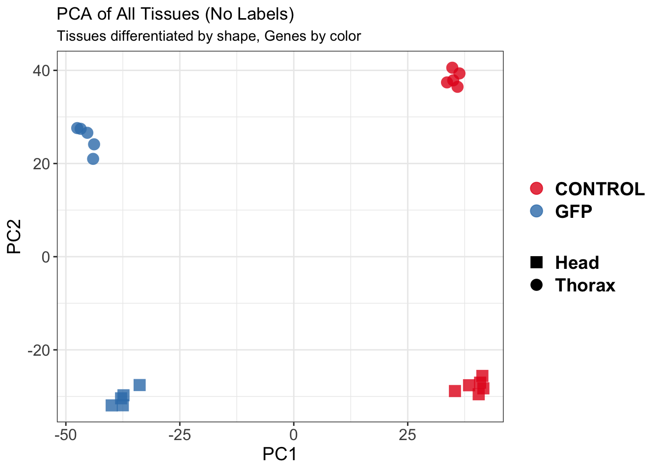
| Version | Author | Date |
|---|---|---|
| 9451c02 | Maeva TECHER | 2025-03-03 |
$WithLabel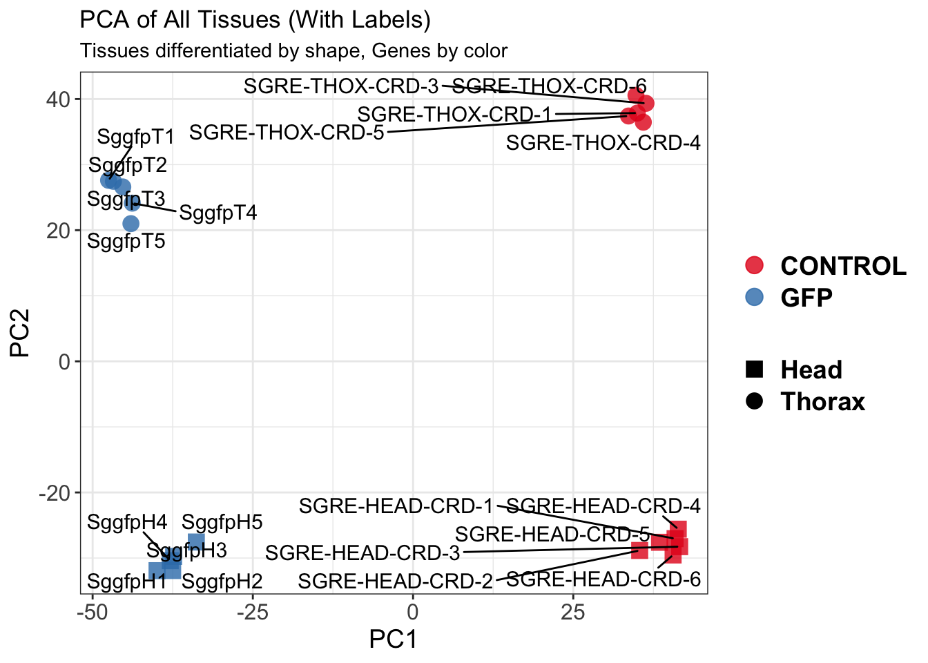
| Version | Author | Date |
|---|---|---|
| 9451c02 | Maeva TECHER | 2025-03-03 |
The PCA plot shows clear distinction between tissue types, while gene silencing has a large variation within each tissue, and presents no distinct clear groupings for a single gene.
SVA
### SVA analysis to control for technical variation
dat <- counts(dds, normalized = TRUE)
idx <- rowMeans(dat) > 1
dat <- dat[idx, ]
mod <- model.matrix(~ Gene, colData(dds))
mod0 <- model.matrix(~ 1, colData(dds))
svseq <- svaseq(dat, mod, mod0)Number of significant surrogate variables is: 2
Iteration (out of 5 ):1 2 3 4 5 sva_plots <- create_sva_plots(svseq, dds, saveDir, intgroup = c("Tissue", "Gene"), max_sv = 3)
# Show stripcharts in the report
sva_plots$Stripcharts[[1]] # Show first stripchart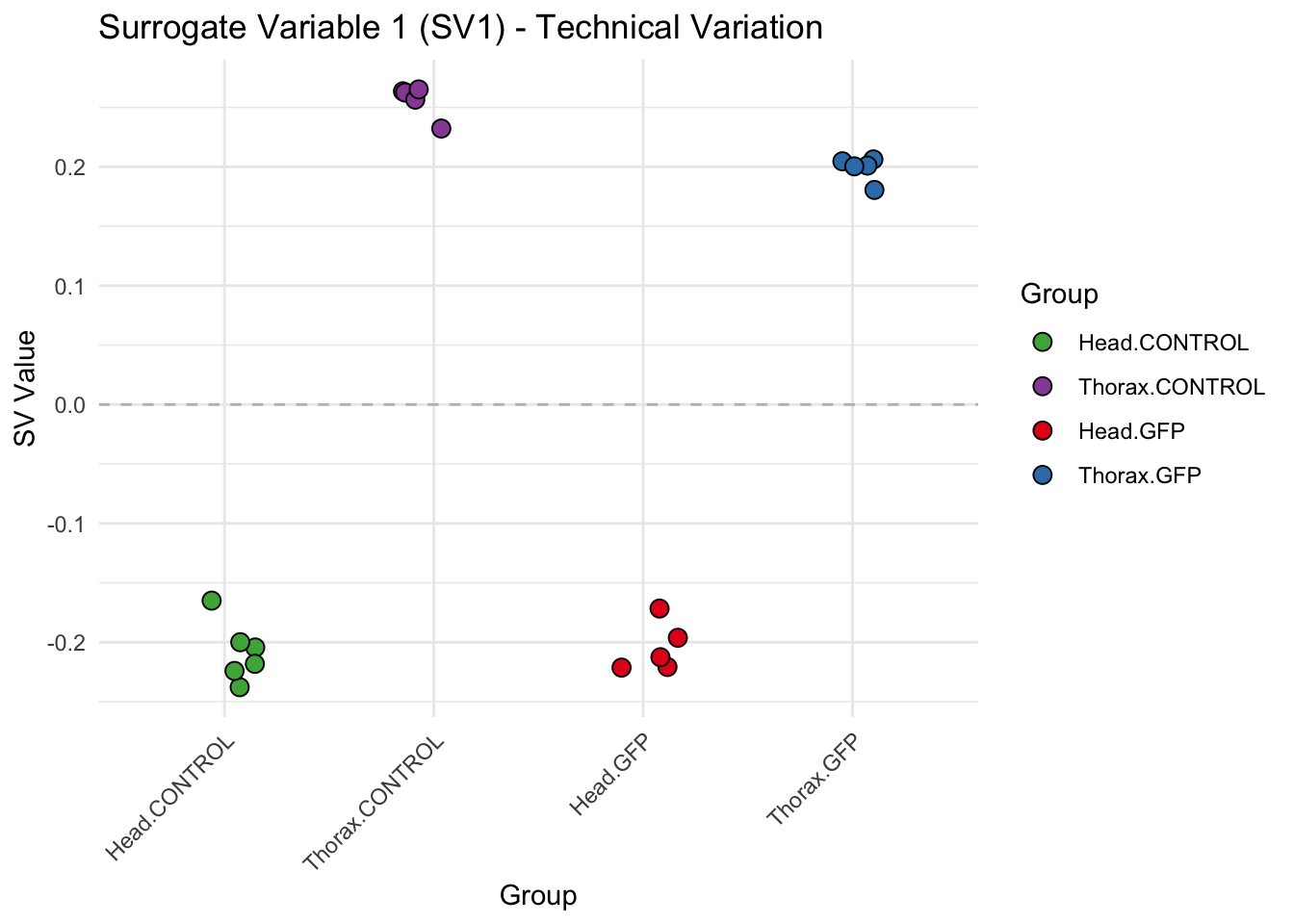
| Version | Author | Date |
|---|---|---|
| 9451c02 | Maeva TECHER | 2025-03-03 |
sva_plots$Stripcharts[[2]] # Show second stripchart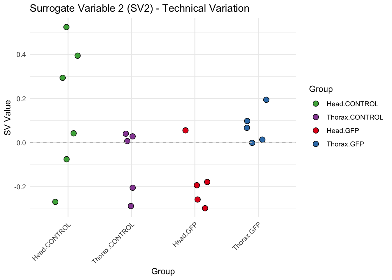
| Version | Author | Date |
|---|---|---|
| 9451c02 | Maeva TECHER | 2025-03-03 |
# Show scatter plots in the report
sva_plots$ScatterPlots[["1_2"]] # Show SV1 vs SV2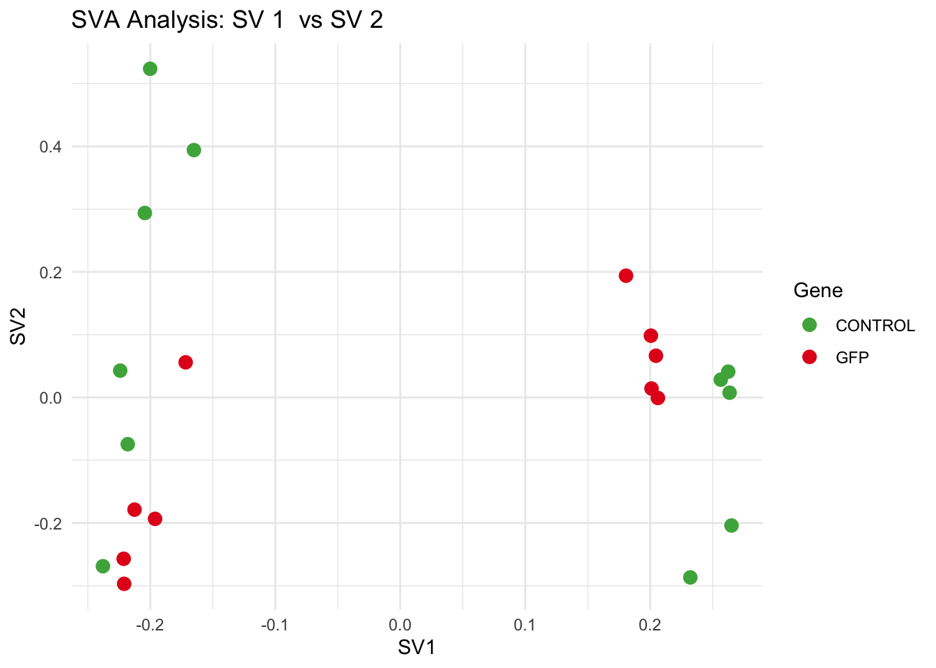
| Version | Author | Date |
|---|---|---|
| 9451c02 | Maeva TECHER | 2025-03-03 |
SV1 is clearly showing an effect of tissue. We rerun the
DESeq2 model but this time including the surrogate variable
SV2 and SV3 as a covariates only, as we know that the modeled variation
is more likely explained by tissue and gene variation rather than batch
effects.
ddssva <- dds
ddssva$SV1 <- svseq$sv[,1]
ddssva$SV2 <- svseq$sv[,2]
design(ddssva) <- ~ SV1 + SV2 + Gene
ddssva$Gene <- relevel(ddssva$Gene, ref = "CONTROL")
smallestGroupSize <- 5
keep <- rowSums(counts(ddssva) >= 10) >= smallestGroupSize
ddssva <- ddssva[keep,]
ddssva <- DESeq(ddssva)
ddssva <- ddssva[which(mcols(ddssva)$betaConv),] # remove non converging rows
### Extract results
message("Available contrasts are: ", paste(resultsNames(ddssva), collapse = ", "))
gfp <- results(ddssva, contrast = c("Gene", "GFP", "CONTROL"), alpha = 0.05)Volcano plots and Heatmaps
# Define contrast_sets
gfp_samples <- c("SGRE-HEAD-CRD-1","SGRE-HEAD-CRD-2","SGRE-HEAD-CRD-3","SGRE-HEAD-CRD-4","SGRE-HEAD-CRD-5",
"SGRE-HEAD-CRD-6","SggfpH1","SggfpH2","SggfpH3","SggfpH4","SggfpH5", "SGRE-THOX-CRD-1","SGRE-THOX-CRD-3","SGRE-THOX-CRD-4","SGRE-THOX-CRD-5",
"SGRE-THOX-CRD-6", "SggfpT1","SggfpT2","SggfpT3","SggfpT4","SggfpT5")
# Run full analysis
gfp_plots <- visualize_data_nopng(gfp, "GFP_vs_CONTROL", gfp_samples)
gfp_plots$volcano; gfp_plots$heatmap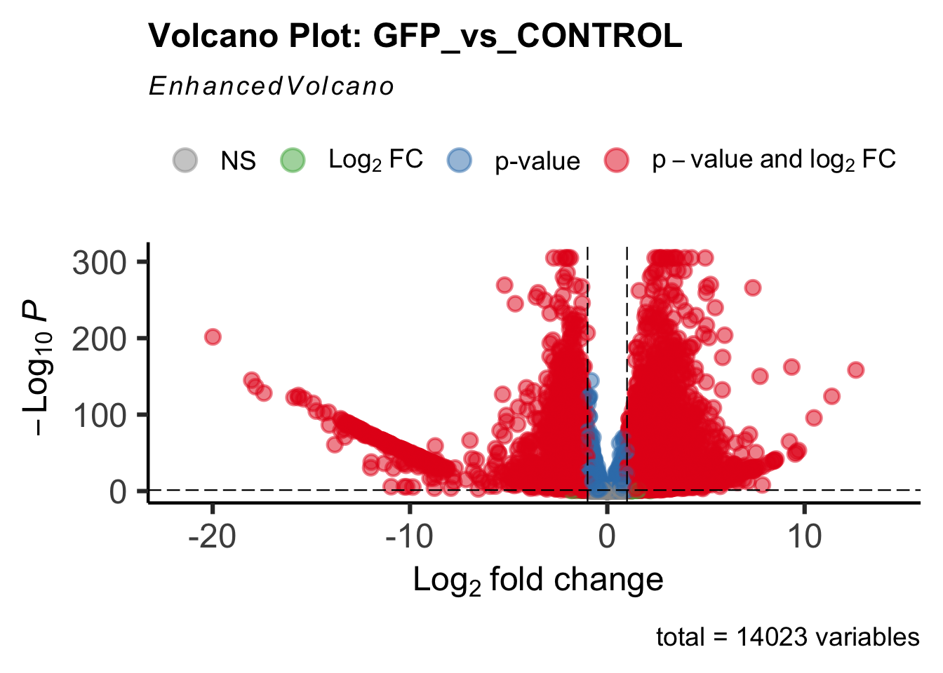
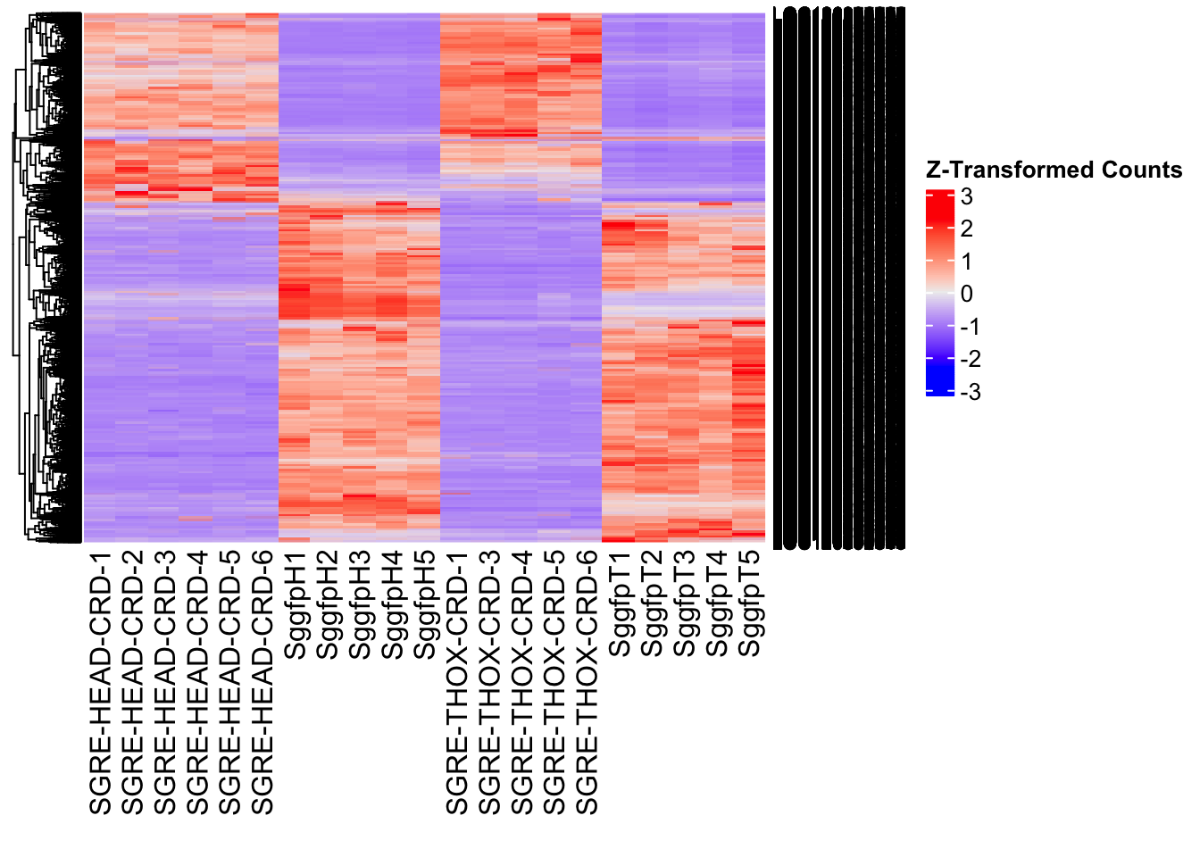
| Version | Author | Date |
|---|---|---|
| 9451c02 | Maeva TECHER | 2025-03-03 |
DEG tables
The following tables show the genes differentially expressed with at least an absolute log2fold change of > 1 considering all tissues together. Considering GFP as the reference state, upregulated genes in knockdown treatment in red and downregulated genes in knockdown treatment in blue. You can search for a gene of interest by writting a LOCID or description in the search bar or sort by column.
# Generate tables for each contrast
table_gfp <- generate_deg_table(ddssva, "Gene_GFP_vs_CONTROL", allspecies_df)
out of 14023 with nonzero total read count
adjusted p-value < 0.05
LFC > 0 (up) : 7238, 52%
LFC < 0 (down) : 4806, 34%
outliers [1] : 0, 0%
low counts [2] : 0, 0%
(mean count < 1)
[1] see 'cooksCutoff' argument of ?results
[2] see 'independentFiltering' argument of ?resultsTotal DEGs p-value < 0.05 and absolute logFoldChange > 1: 8339LFC > 1 (up) : 5423 (65.03%)LFC < -1 (down) : 2916 (34.97%)table_gfp$kable_tableSummary and Overlap
# Summarize DEGs for all contrasts
deg_summary <- bind_rows(
summarize_deg_counts(table_gfp, "GFP vs CONTROL")
)
# Display table using kable with styling
deg_summary %>%
kable("html", escape = FALSE, col.names = gsub("_", " ", names(.))) %>%
kable_styling("striped", full_width = TRUE) %>%
column_spec(2, color = "red", bold = TRUE) %>% # Upregulated in red
column_spec(3, color = "blue", bold = TRUE) %>% # Downregulated in blue
add_header_above(c("Summary of DEGs" = 3)) %>%
row_spec(0, bold = TRUE)| Contrast | Upregulated | Downregulated |
|---|---|---|
| GFP vs CONTROL | 5402 | 2901 |
# Define the list of RNAi contrasts
contrast_list <- c("GFP_vs_CONTROL")
# Initialize empty lists for storing Head-specific DEGs for each contrast
venn_data_up <- list()
venn_data_down <- list()
venn_data_all <- list()
# Function to load Head-specific DEGs for a given set of contrasts
load_deg_contrasts_head <- function(contrast_list) {
degs_up <- list()
degs_down <- list()
degs_all <- list()
for (contrast in contrast_list) {
deg_file <- file.path(workDir, "DEG_results/RNAi/All_GFP_no_rRNA/", contrast, paste0("DEG_sigresults_", contrast, ".csv"))
if (!file.exists(deg_file)) {
message(paste("File missing for contrast:", contrast))
next # Skip if the file doesn't exist
}
deg_data <- read.csv(deg_file, stringsAsFactors = FALSE)
# Convert row names to a column if necessary
if ("X" %in% colnames(deg_data)) {
colnames(deg_data)[colnames(deg_data) == "X"] <- "GeneID"
}
# Check if data is empty
if (nrow(deg_data) == 0) {
message(paste("No data for contrast:", contrast))
next
}
# Select significant DEGs (Up, Down, All)
degs_up[[contrast]] <- deg_data %>%
filter(padj < 0.05 & log2FoldChange >= 1) %>%
pull(GeneID) # Extract GeneID column
degs_down[[contrast]] <- deg_data %>%
filter(padj < 0.05 & log2FoldChange <= -1) %>%
pull(GeneID) # Extract GeneID column
degs_all[[contrast]] <- deg_data %>%
filter(padj < 0.05 & abs(log2FoldChange) >= 1) %>%
pull(GeneID) # Extract GeneID column
}
return(list(up = degs_up, down = degs_down, all = degs_all))
}
# Load DEG data for the defined contrasts (Head tissue only)
venn_data_contrasts <- load_deg_contrasts_head(contrast_list)
# Prepare the data for the Venn diagrams
venn_data_up <- venn_data_contrasts$up
venn_data_down <- venn_data_contrasts$down
venn_data_all <- venn_data_contrasts$allHead tissue
saveDir <- paste0(workDir,"/DEG_results/RNAi/Head_GFP_no_rRNA")
dir.create(saveDir)
### Prepare Sample CSV file #####
samples <- read.delim(file.path(workDir, "list/RNAi/Head_RNAi_GFPCRDsample_list.csv"), sep = ",", row.names = 1, header = TRUE)
files <- file.path(workDir, "readcounts/RNAi/", samples$Tissue, samples$Filename)
names(files) <- row.names(samples)
if (all(file.exists(files))) {
message("All the files exist!")
} else {
warning("Some files are missing!")
}All the files exist!### **Standardized Count Matrix Creation**
# Extract all gene lists first
gene_lists <- map(files, function(sample) {
fread(sample, sep = "\t", header = FALSE)[, 1] # Extract Gene IDs (column 1)
})
# Get a unique set of all gene IDs across all samples
all_genes <- unique(unlist(gene_lists))
# Create a named list to store count data with standardized rows
cts_list <- map(files, function(sample) {
data_count <- fread(sample, sep = "\t", header = FALSE)
col_name <- gsub("_counts.txt", "", basename(sample)) # Clean sample name
# Convert to data frame with correct column names
data_count <- setNames(data.frame(data_count[, 1:2]), c("GeneID", col_name))
# Ensure all gene IDs are present (fill missing values with 0)
data_count <- full_join(data.frame(GeneID = all_genes), data_count, by = "GeneID") %>%
mutate(across(where(is.numeric), ~ replace_na(., 0))) # Fill NA with 0
return(data_count)
})
# Merge all samples based on GeneID
cts <- reduce(cts_list, full_join, by = "GeneID")
# Convert to matrix for DESeq2
cts_matrix <- as.matrix(cts[, -1]) # Remove GeneID column for count matrix
rownames(cts_matrix) <- cts$GeneID # Set GeneID as rownames
rm(cts_list) # Free memoryWhile for bulk RNAseq on head and thorax for all species, the DEGs model was made between isolated and crowded individuals (with isolated as the reference state), here, the DEG analysis will be carried between GFP knock-down nymphs (as reference state) vs Hexamerins / Juvenile Hormones / Inositol / Uncharacterized proteins.
### Build DESeq2 Object
dds <- DESeqDataSetFromMatrix(countData = cts_matrix,
colData = samples,
design = ~ Gene)
dds$Gene <- relevel(dds$Gene, ref = "CONTROL")
smallestGroupSize <- 5
keep <- rowSums(counts(dds) >= 10) >= smallestGroupSize
dds <- dds[keep,]
loci_to_exclude <- readLines(file.path(workDir, "list/excluded_loci/gregaria_rrna_list.txt"))
dds <- dds[!(rownames(dds) %in% loci_to_exclude), ]
dds <- DESeq(dds)Normalization and PCA
# Plot PCA and investigate quality metrics
vsd <- vst(dds, blind = TRUE)
# Perform PCA
pca_data <- plotPCA(vsd, intgroup = c("Tissue", "Gene"), returnData = TRUE)
# Define colors for genes (slightly transparent) and shapes for tissues
gene_colors <- scale_color_manual(values = alpha(brewer.pal(n = length(unique(pca_data$Gene)), name = "Set1"), 0.8)) # Points are transparent
tissue_shapes <- scale_shape_manual(values = seq(15, 15 + length(unique(pca_data$Tissue))))
# **PCA without labels**
p_pca_nolabel <- ggplot(pca_data, aes(x = PC1, y = PC2, color = Gene, shape = Tissue)) +
geom_point(size = 4) +
gene_colors +
tissue_shapes +
theme_bw() +
theme(legend.title = element_blank(),
legend.text = element_text(face = "bold", size = 14),
axis.text = element_text(size = 12),
axis.title = element_text(size = 14)) +
ggtitle("PCA of All Tissues (No Labels)", subtitle = "Tissues differentiated by shape, Genes by color")
# Save PCA without labels
ggsave(paste0(saveDir, "/PCA_Tissue_Gene_NoLabel.png"), plot = p_pca_nolabel, width = 10, height = 10, dpi = 600, device = "png")
# **PCA with labels**
p_pca_label <- ggplot(pca_data, aes(x = PC1, y = PC2, color = Gene, shape = Tissue)) +
geom_point(size = 4) +
geom_text_repel(aes(label = name), size = 4, color = "black", max.overlaps = 20) + # Labels are fully visible
gene_colors +
tissue_shapes +
theme_bw() +
theme(legend.title = element_blank(),
legend.text = element_text(face = "bold", size = 14),
axis.text = element_text(size = 12),
axis.title = element_text(size = 14)) +
ggtitle("PCA of All Tissues (With Labels)", subtitle = "Tissues differentiated by shape, Genes by color")
# Save PCA with labels
ggsave(paste0(saveDir, "/PCA_Tissue_Gene_Label.png"), plot = p_pca_label, width = 10, height = 10, dpi = 600, device = "png")
# **Return plots for knitr/RMarkdown**
list(NoLabel = p_pca_nolabel, WithLabel = p_pca_label)$NoLabel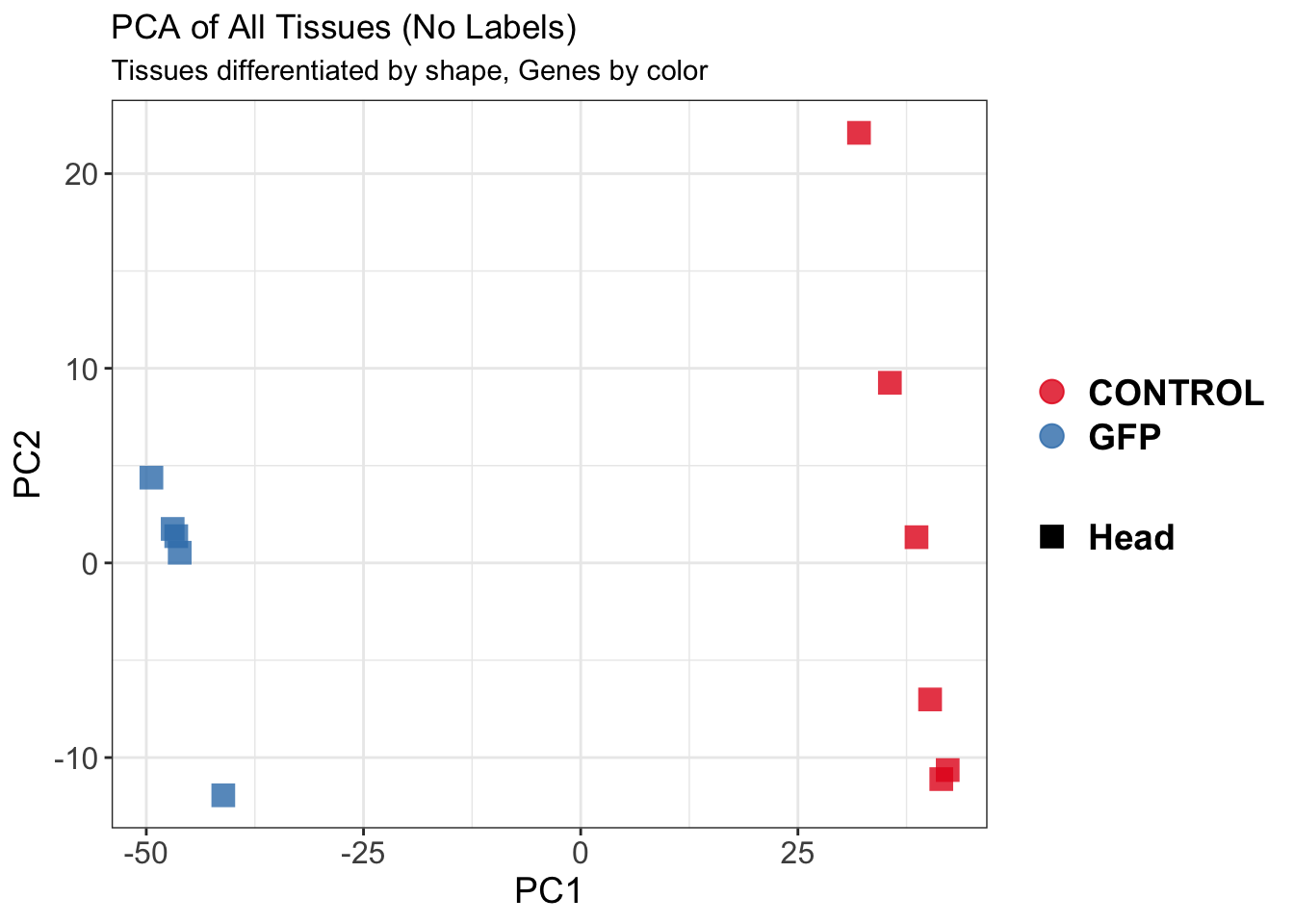
| Version | Author | Date |
|---|---|---|
| 9451c02 | Maeva TECHER | 2025-03-03 |
$WithLabel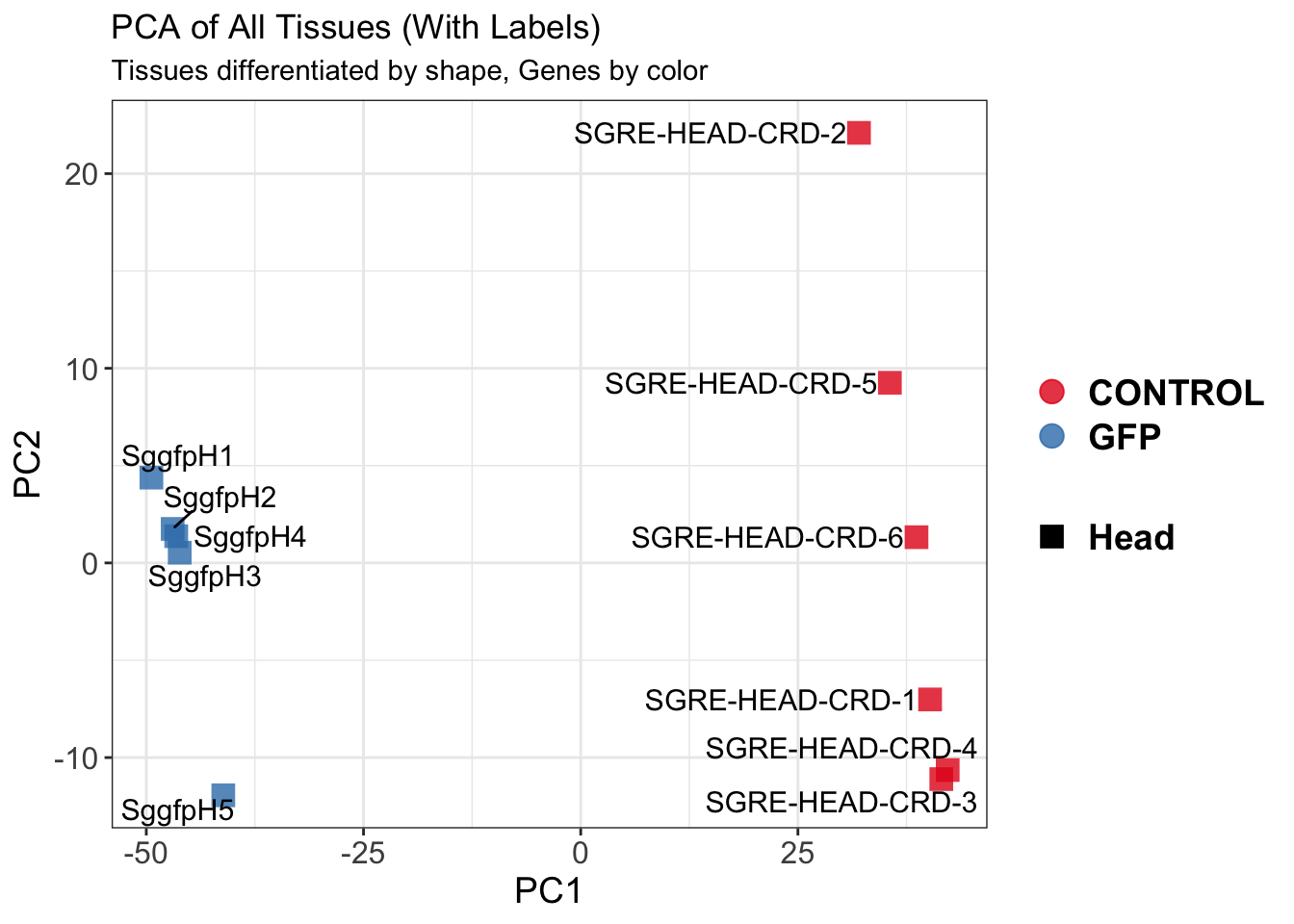
| Version | Author | Date |
|---|---|---|
| 9451c02 | Maeva TECHER | 2025-03-03 |
The PCA plot shows clear distinction between tissue types, while gene silencing has a large variation within each tissue, and presents no distinct clear groupings for a single gene.
SVA
### SVA analysis to control for technical variation
dat <- counts(dds, normalized = TRUE)
idx <- rowMeans(dat) > 1
dat <- dat[idx, ]
mod <- model.matrix(~ Gene, colData(dds))
mod0 <- model.matrix(~ 1, colData(dds))
svseq <- svaseq(dat, mod, mod0)Number of significant surrogate variables is: 4
Iteration (out of 5 ):1 2 3 4 5 sva_plots <- create_sva_plots(svseq, dds, saveDir, intgroup = c("Tissue", "Gene"), max_sv = 7)
# Show stripcharts in the report
sva_plots$Stripcharts[[1]] # Show first stripchart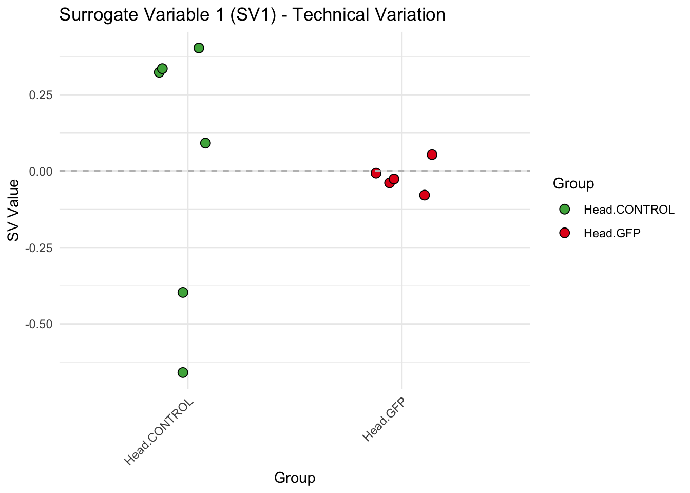
| Version | Author | Date |
|---|---|---|
| 9451c02 | Maeva TECHER | 2025-03-03 |
sva_plots$Stripcharts[[2]] # Show second stripchart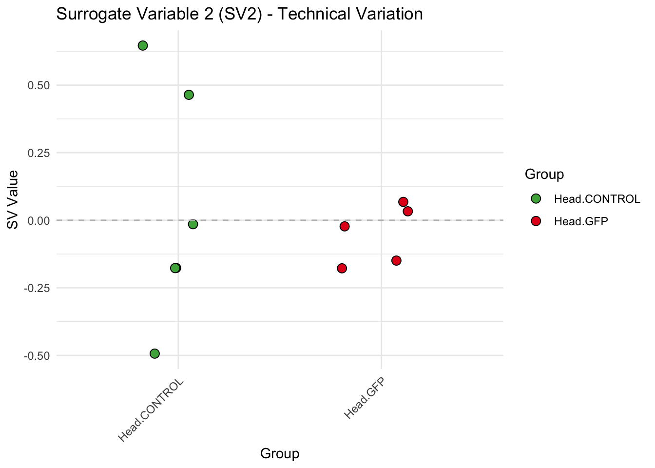
| Version | Author | Date |
|---|---|---|
| 9451c02 | Maeva TECHER | 2025-03-03 |
sva_plots$Stripcharts[[3]] # Show third stripchart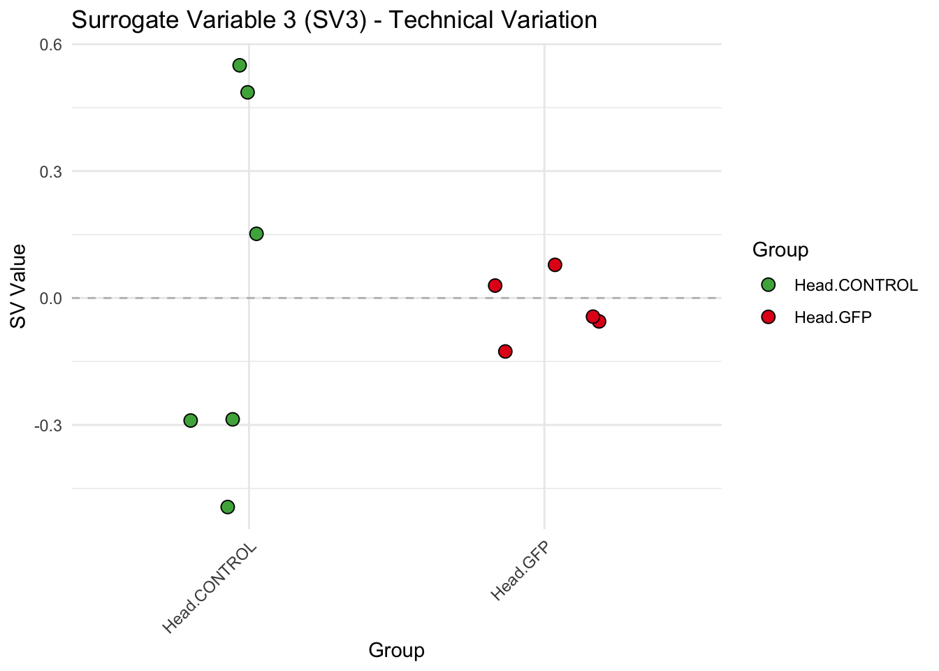
| Version | Author | Date |
|---|---|---|
| 9451c02 | Maeva TECHER | 2025-03-03 |
sva_plots$Stripcharts[[4]] 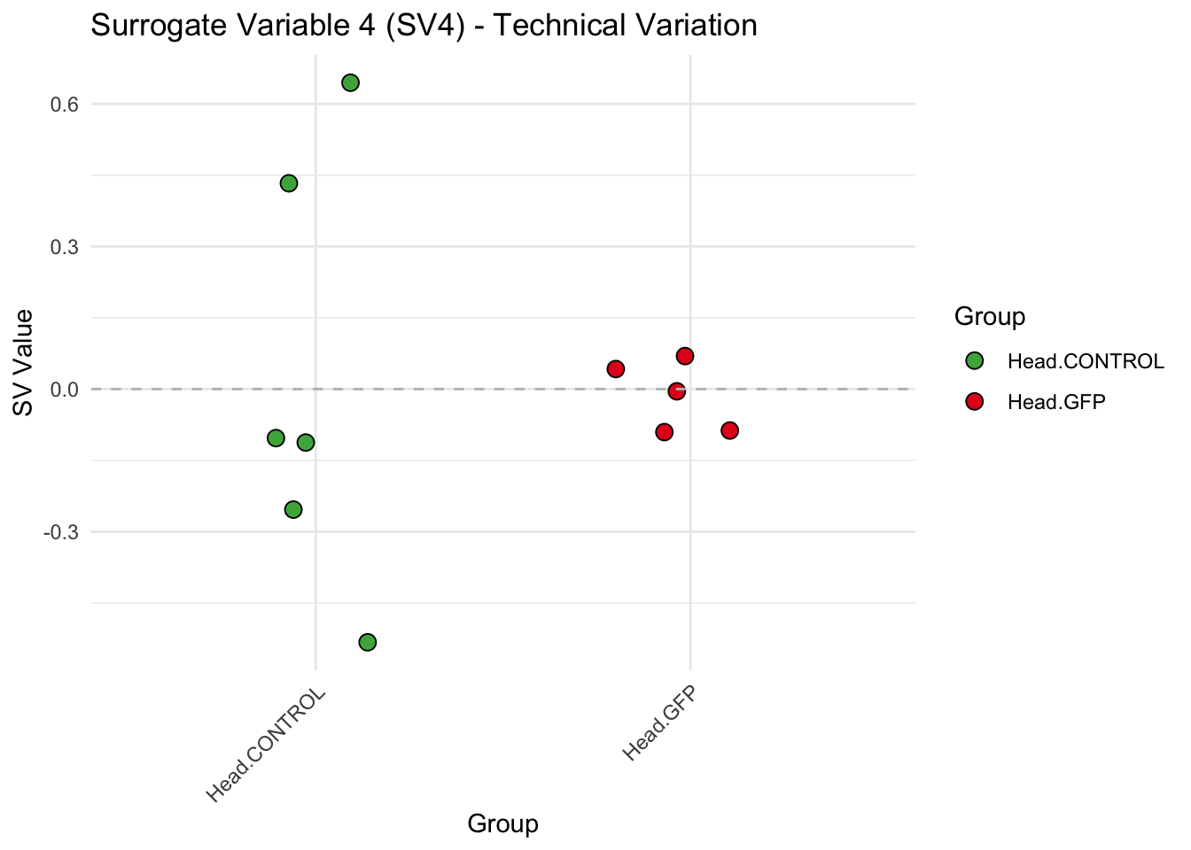
| Version | Author | Date |
|---|---|---|
| 9451c02 | Maeva TECHER | 2025-03-03 |
# Show scatter plots in the report
sva_plots$ScatterPlots[["1_2"]] # Show SV1 vs SV2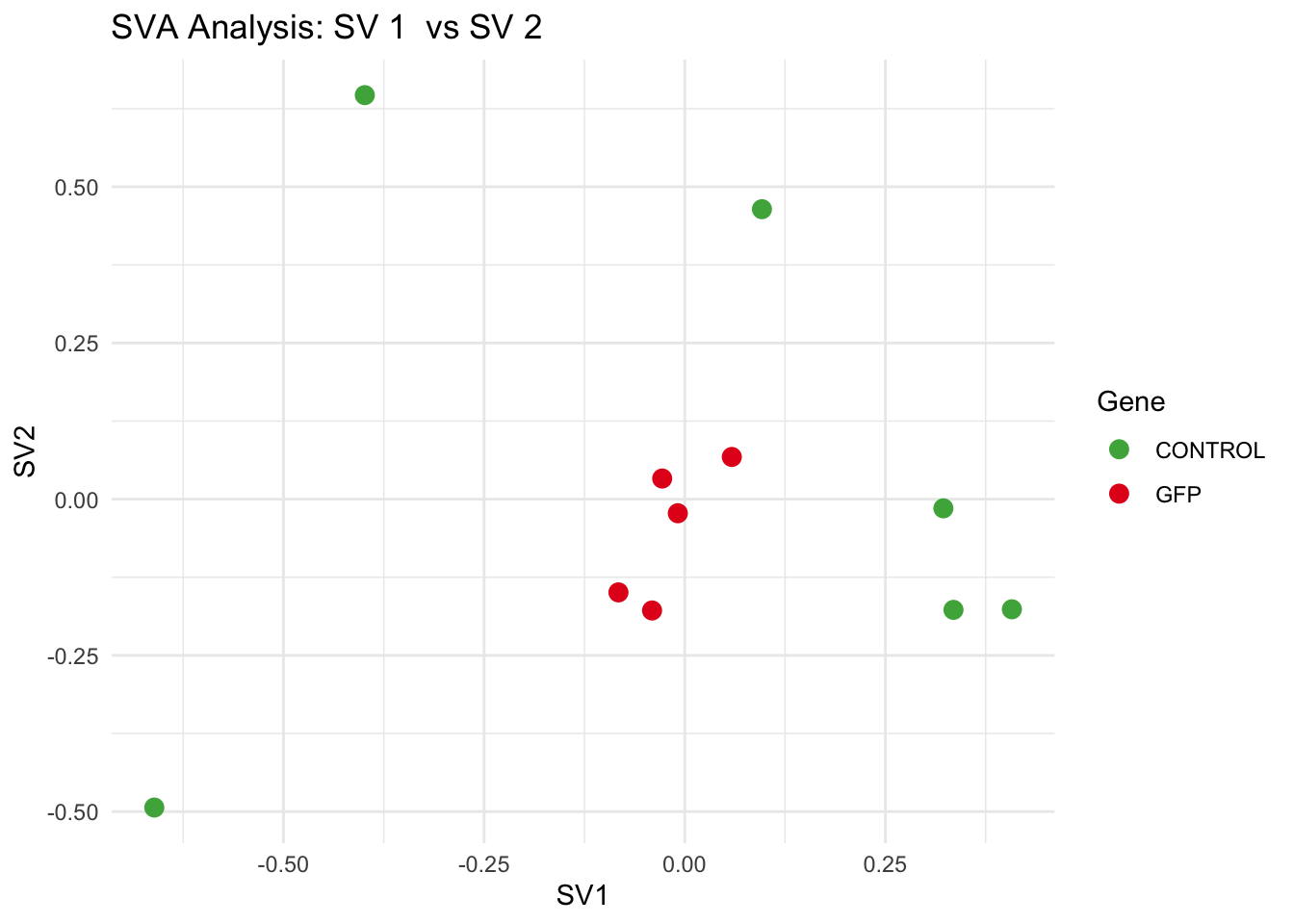
| Version | Author | Date |
|---|---|---|
| 9451c02 | Maeva TECHER | 2025-03-03 |
sva_plots$ScatterPlots[["1_3"]] # Show SV1 vs SV3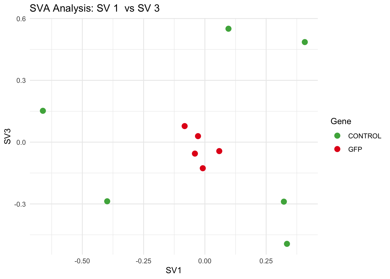
| Version | Author | Date |
|---|---|---|
| 9451c02 | Maeva TECHER | 2025-03-03 |
sva_plots$ScatterPlots[["2_3"]] # Show SV2 vs SV3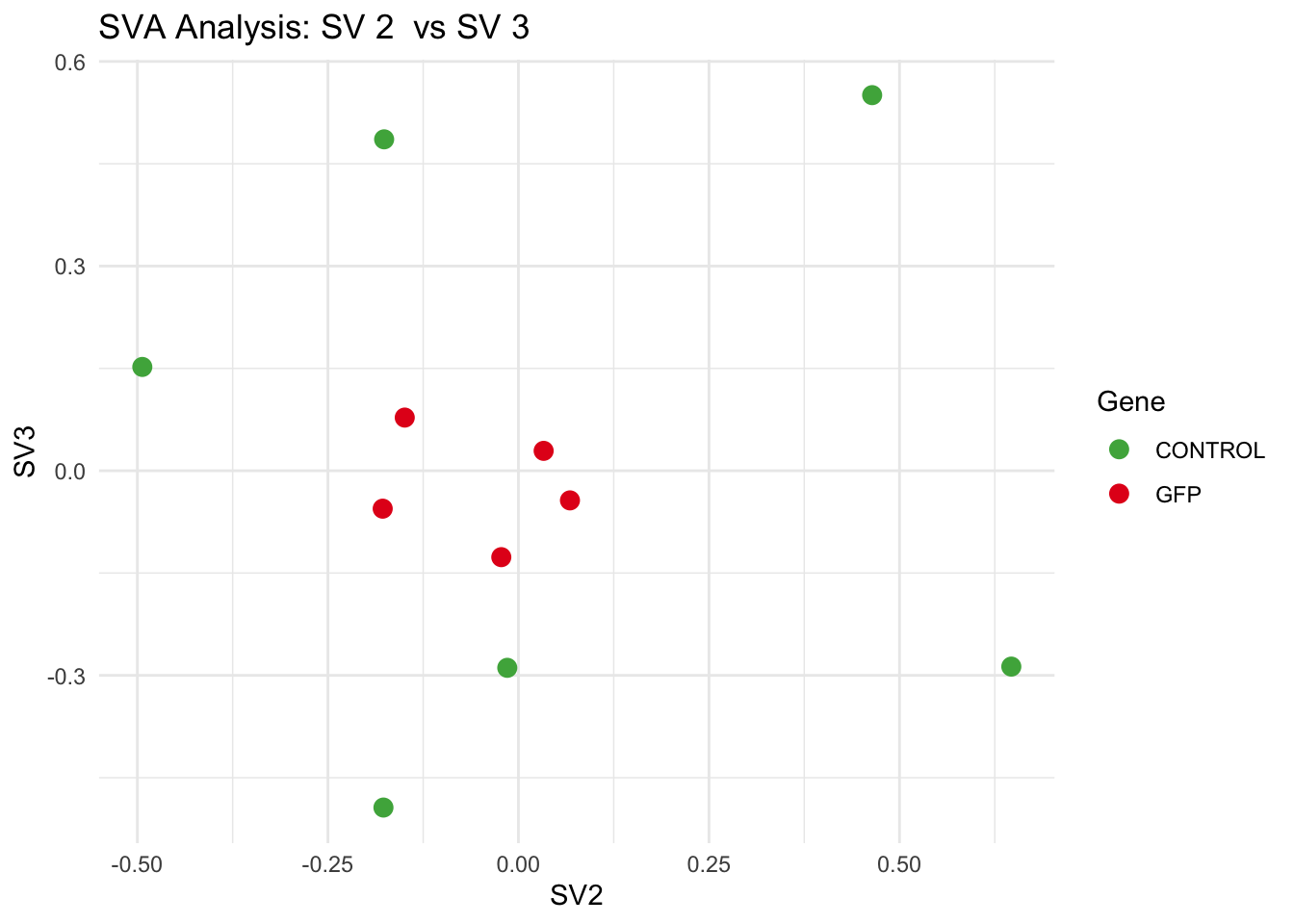
| Version | Author | Date |
|---|---|---|
| 9451c02 | Maeva TECHER | 2025-03-03 |
SV1 is clearly showing an effect of tissue. We rerun the
DESeq2 model but this time including the surrogate variable
SV2 and SV3 as a covariates only, as we know that the modeled variation
is more likely explained by tissue and gene variation rather than batch
effects.
ddssva <- dds
ddssva$SV1 <- svseq$sv[,1]
ddssva$SV2 <- svseq$sv[,2]
ddssva$SV3 <- svseq$sv[,3]
ddssva$SV4 <- svseq$sv[,4]
design(ddssva) <- ~ SV1 + SV2 + SV3 + SV4 + Gene
ddssva$Gene <- relevel(ddssva$Gene, ref = "CONTROL")
smallestGroupSize <- 5
keep <- rowSums(counts(ddssva) >= 10) >= smallestGroupSize
ddssva <- ddssva[keep,]
ddssva <- DESeq(ddssva)
ddssva <- ddssva[which(mcols(ddssva)$betaConv),] # remove non converging rows
### Extract results
message("Available contrasts are: ", paste(resultsNames(ddssva), collapse = ", "))
gfp <- results(ddssva, contrast = c("Gene", "GFP", "CONTROL"), alpha = 0.05)Volcano plots and Heatmaps
# Define contrast_sets
gfp_samples <- c("SGRE-HEAD-CRD-1","SGRE-HEAD-CRD-2","SGRE-HEAD-CRD-3","SGRE-HEAD-CRD-4","SGRE-HEAD-CRD-5",
"SGRE-HEAD-CRD-6","SggfpH1","SggfpH2","SggfpH3","SggfpH4","SggfpH5")
# Run full analysis
gfp_plots <- visualize_data_nopng(gfp, "GFP_vs_CONTROL", gfp_samples)
gfp_plots$volcano; gfp_plots$heatmap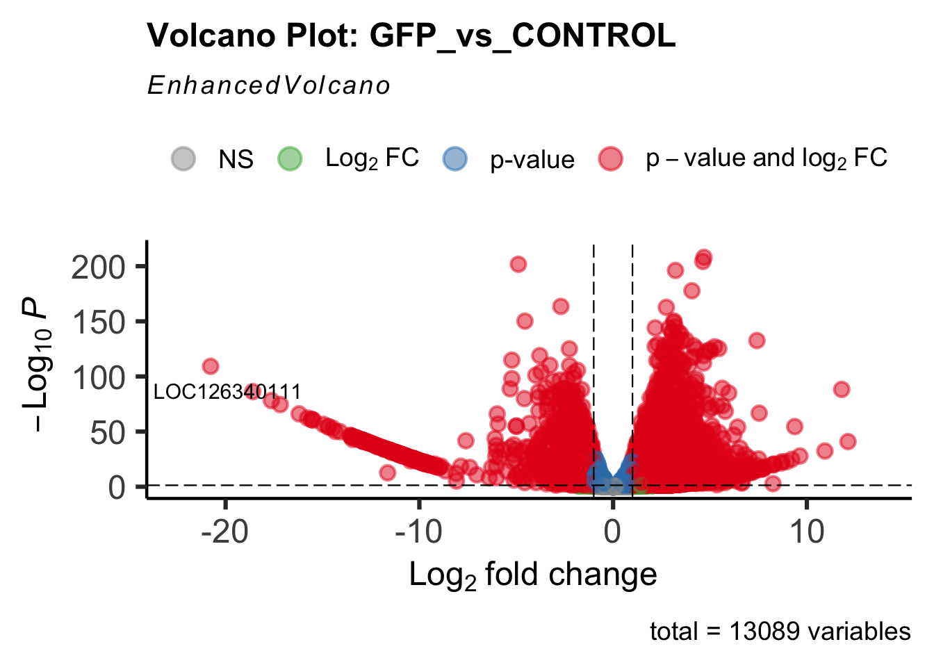
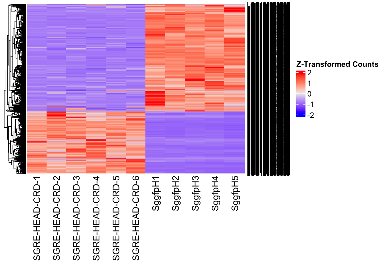
| Version | Author | Date |
|---|---|---|
| 9451c02 | Maeva TECHER | 2025-03-03 |
DEG tables
The following tables show the genes differentially expressed with at least an absolute log2fold change of > 1 considering Head tissues only. Considering GFP as the reference state, upregulated genes in knockdown treatment in red and downregulated genes in knockdown treatment in blue. You can search for a gene of interest by writting a LOCID or description in the search bar or sort by column.
# Generate tables for each contrast
table_gfp <- generate_deg_table(ddssva, "Gene_GFP_vs_CONTROL", allspecies_df)
out of 13089 with nonzero total read count
adjusted p-value < 0.05
LFC > 0 (up) : 6064, 46%
LFC < 0 (down) : 4262, 33%
outliers [1] : 0, 0%
low counts [2] : 0, 0%
(mean count < 1)
[1] see 'cooksCutoff' argument of ?results
[2] see 'independentFiltering' argument of ?resultsTotal DEGs p-value < 0.05 and absolute logFoldChange > 1: 7414LFC > 1 (up) : 4705 (63.46%)LFC < -1 (down) : 2709 (36.54%)table_gfp$kable_tableSummary and Overlap
# Summarize DEGs for all contrasts
deg_summary <- bind_rows(
summarize_deg_counts(table_gfp, "GFP vs CONTROL")
)
# Display table using kable with styling
deg_summary %>%
kable("html", escape = FALSE, col.names = gsub("_", " ", names(.))) %>%
kable_styling("striped", full_width = TRUE) %>%
column_spec(2, color = "red", bold = TRUE) %>% # Upregulated in red
column_spec(3, color = "blue", bold = TRUE) %>% # Downregulated in blue
add_header_above(c("Summary of DEGs" = 3)) %>%
row_spec(0, bold = TRUE)| Contrast | Upregulated | Downregulated |
|---|---|---|
| GFP vs CONTROL | 4681 | 2687 |
# Define the list of RNAi contrasts
contrast_list <- c("GFP_vs_CONTROL")
# Initialize empty lists for storing Head-specific DEGs for each contrast
venn_data_up <- list()
venn_data_down <- list()
venn_data_all <- list()
# Function to load Head-specific DEGs for a given set of contrasts
load_deg_contrasts_head <- function(contrast_list) {
degs_up <- list()
degs_down <- list()
degs_all <- list()
for (contrast in contrast_list) {
deg_file <- file.path(workDir, "DEG_results/RNAi/Head_GFP_no_rRNA/", contrast, paste0("DEG_sigresults_", contrast, ".csv"))
if (!file.exists(deg_file)) {
message(paste("File missing for contrast:", contrast))
next # Skip if the file doesn't exist
}
deg_data <- read.csv(deg_file, stringsAsFactors = FALSE)
# Convert row names to a column if necessary
if ("X" %in% colnames(deg_data)) {
colnames(deg_data)[colnames(deg_data) == "X"] <- "GeneID"
}
# Check if data is empty
if (nrow(deg_data) == 0) {
message(paste("No data for contrast:", contrast))
next
}
# Select significant DEGs (Up, Down, All)
degs_up[[contrast]] <- deg_data %>%
filter(padj < 0.05 & log2FoldChange >= 1) %>%
pull(GeneID) # Extract GeneID column
degs_down[[contrast]] <- deg_data %>%
filter(padj < 0.05 & log2FoldChange <= -1) %>%
pull(GeneID) # Extract GeneID column
degs_all[[contrast]] <- deg_data %>%
filter(padj < 0.05 & abs(log2FoldChange) >= 1) %>%
pull(GeneID) # Extract GeneID column
}
return(list(up = degs_up, down = degs_down, all = degs_all))
}
# Load DEG data for the defined contrasts (Head tissue only)
venn_data_contrasts <- load_deg_contrasts_head(contrast_list)
# Prepare the data for the Venn diagrams
venn_data_up <- venn_data_contrasts$up
venn_data_down <- venn_data_contrasts$down
venn_data_all <- venn_data_contrasts$allThorax tissue
saveDir <- paste0(workDir,"/DEG_results/RNAi/Thorax_GFP_no_rRNA")
dir.create(saveDir)
### Prepare Sample CSV file #####
samples <- read.delim(file.path(workDir, "list/RNAi/Thorax_RNAi_GFPCRDsample_list.csv"), sep = ",", row.names = 1, header = TRUE)
files <- file.path(workDir, "readcounts/RNAi/", samples$Tissue, samples$Filename)
names(files) <- row.names(samples)
if (all(file.exists(files))) {
message("All the files exist!")
} else {
warning("Some files are missing!")
}All the files exist!### **Standardized Count Matrix Creation**
# Extract all gene lists first
gene_lists <- map(files, function(sample) {
fread(sample, sep = "\t", header = FALSE)[, 1] # Extract Gene IDs (column 1)
})
# Get a unique set of all gene IDs across all samples
all_genes <- unique(unlist(gene_lists))
# Create a named list to store count data with standardized rows
cts_list <- map(files, function(sample) {
data_count <- fread(sample, sep = "\t", header = FALSE)
col_name <- gsub("_counts.txt", "", basename(sample)) # Clean sample name
# Convert to data frame with correct column names
data_count <- setNames(data.frame(data_count[, 1:2]), c("GeneID", col_name))
# Ensure all gene IDs are present (fill missing values with 0)
data_count <- full_join(data.frame(GeneID = all_genes), data_count, by = "GeneID") %>%
mutate(across(where(is.numeric), ~ replace_na(., 0))) # Fill NA with 0
return(data_count)
})
# Merge all samples based on GeneID
cts <- reduce(cts_list, full_join, by = "GeneID")
# Convert to matrix for DESeq2
cts_matrix <- as.matrix(cts[, -1]) # Remove GeneID column for count matrix
rownames(cts_matrix) <- cts$GeneID # Set GeneID as rownames
rm(cts_list) # Free memoryWhile for bulk RNAseq on head and thorax for all species, the DEGs model was made between isolated and crowded individuals (with isolated as the reference state), here, the DEG analysis will be carried between GFP knock-down nymphs (as reference state) vs Hexamerins / Juvenile Hormones / Inositol / Uncharacterized proteins.
### Build DESeq2 Object
dds <- DESeqDataSetFromMatrix(countData = cts_matrix,
colData = samples,
design = ~ Gene)
dds$Gene <- relevel(dds$Gene, ref = "CONTROL")
smallestGroupSize <- 5
keep <- rowSums(counts(dds) >= 10) >= smallestGroupSize
dds <- dds[keep,]
loci_to_exclude <- readLines(file.path(workDir, "list/excluded_loci/gregaria_rrna_list.txt"))
dds <- dds[!(rownames(dds) %in% loci_to_exclude), ]
dds <- DESeq(dds)Normalization and PCA
# Plot PCA and investigate quality metrics
vsd <- vst(dds, blind = TRUE)
# Perform PCA
pca_data <- plotPCA(vsd, intgroup = c("Tissue", "Gene"), returnData = TRUE)
# Define colors for genes (slightly transparent) and shapes for tissues
gene_colors <- scale_color_manual(values = alpha(brewer.pal(n = length(unique(pca_data$Gene)), name = "Set1"), 0.8)) # Points are transparent
tissue_shapes <- scale_shape_manual(values = seq(15, 15 + length(unique(pca_data$Tissue))))
# **PCA without labels**
p_pca_nolabel <- ggplot(pca_data, aes(x = PC1, y = PC2, color = Gene, shape = Tissue)) +
geom_point(size = 4) +
gene_colors +
tissue_shapes +
theme_bw() +
theme(legend.title = element_blank(),
legend.text = element_text(face = "bold", size = 14),
axis.text = element_text(size = 12),
axis.title = element_text(size = 14)) +
ggtitle("PCA of All Tissues (No Labels)", subtitle = "Tissues differentiated by shape, Genes by color")
# Save PCA without labels
ggsave(paste0(saveDir, "/PCA_Tissue_Gene_NoLabel.png"), plot = p_pca_nolabel, width = 10, height = 10, dpi = 600, device = "png")
# **PCA with labels**
p_pca_label <- ggplot(pca_data, aes(x = PC1, y = PC2, color = Gene, shape = Tissue)) +
geom_point(size = 4) +
geom_text_repel(aes(label = name), size = 4, color = "black", max.overlaps = 20) + # Labels are fully visible
gene_colors +
tissue_shapes +
theme_bw() +
theme(legend.title = element_blank(),
legend.text = element_text(face = "bold", size = 14),
axis.text = element_text(size = 12),
axis.title = element_text(size = 14)) +
ggtitle("PCA of All Tissues (With Labels)", subtitle = "Tissues differentiated by shape, Genes by color")
# Save PCA with labels
ggsave(paste0(saveDir, "/PCA_Tissue_Gene_Label.png"), plot = p_pca_label, width = 10, height = 10, dpi = 600, device = "png")
# **Return plots for knitr/RMarkdown**
list(NoLabel = p_pca_nolabel, WithLabel = p_pca_label)$NoLabel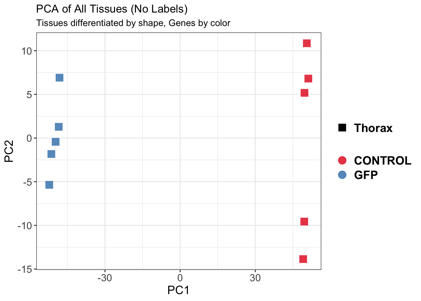
| Version | Author | Date |
|---|---|---|
| 9451c02 | Maeva TECHER | 2025-03-03 |
$WithLabel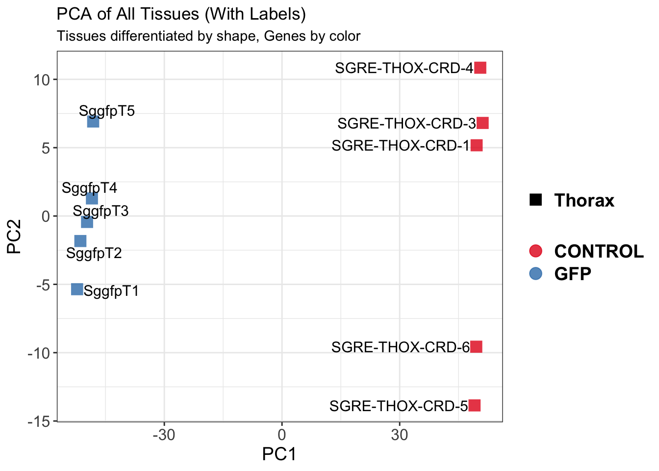
| Version | Author | Date |
|---|---|---|
| 9451c02 | Maeva TECHER | 2025-03-03 |
The PCA plot shows clear distinction between tissue types, while gene silencing has a large variation within each tissue, and presents no distinct clear groupings for a single gene.
SVA
### SVA analysis to control for technical variation
dat <- counts(dds, normalized = TRUE)
idx <- rowMeans(dat) > 1
dat <- dat[idx, ]
mod <- model.matrix(~ Gene, colData(dds))
mod0 <- model.matrix(~ 1, colData(dds))
svseq <- svaseq(dat, mod, mod0)Number of significant surrogate variables is: 2
Iteration (out of 5 ):1 2 3 4 5 sva_plots <- create_sva_plots(svseq, dds, saveDir, intgroup = c("Tissue", "Gene"), max_sv = 6)
# Show stripcharts in the report
sva_plots$Stripcharts[[1]] # Show first stripchart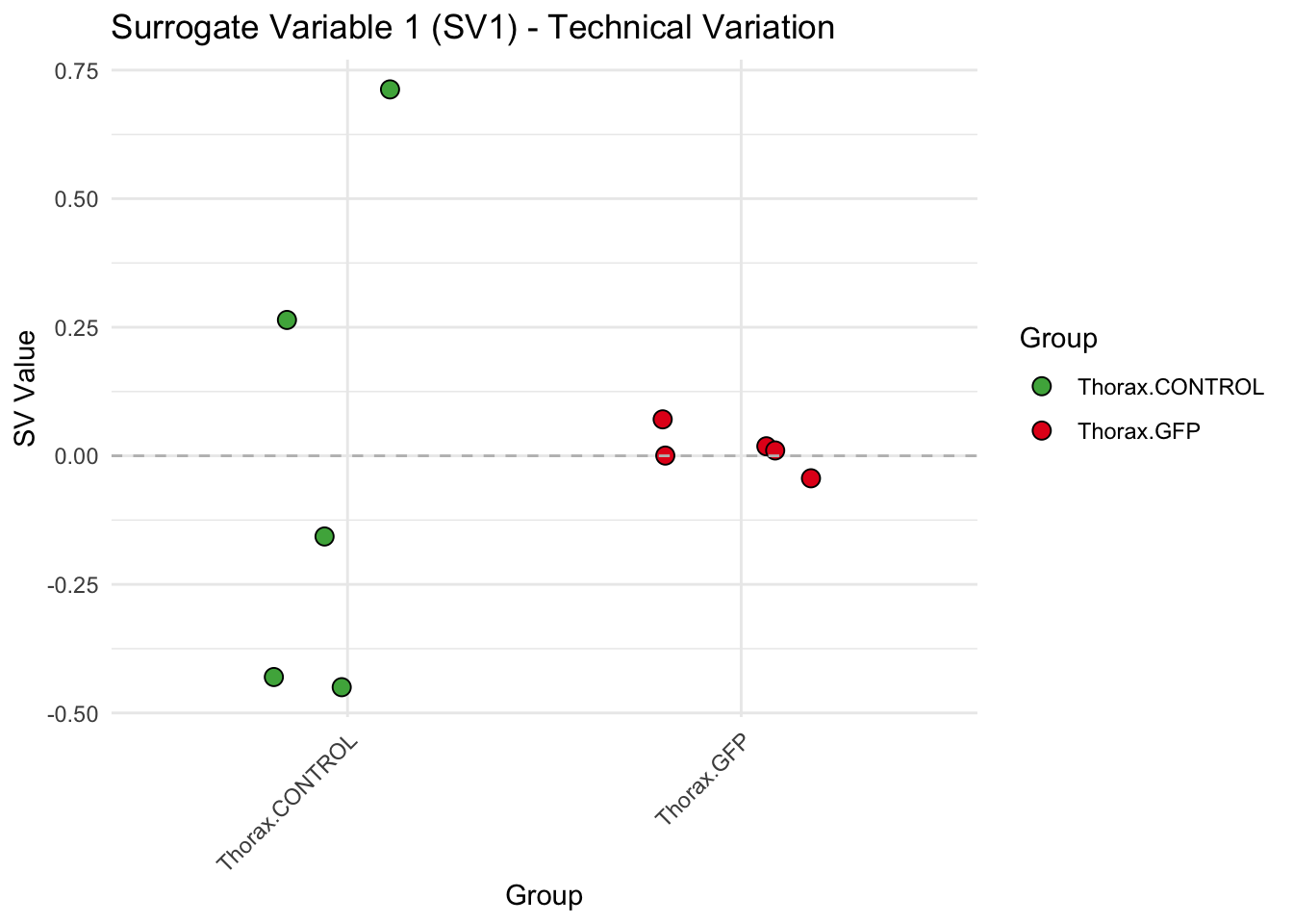
| Version | Author | Date |
|---|---|---|
| 9451c02 | Maeva TECHER | 2025-03-03 |
sva_plots$Stripcharts[[2]] # Show second stripchart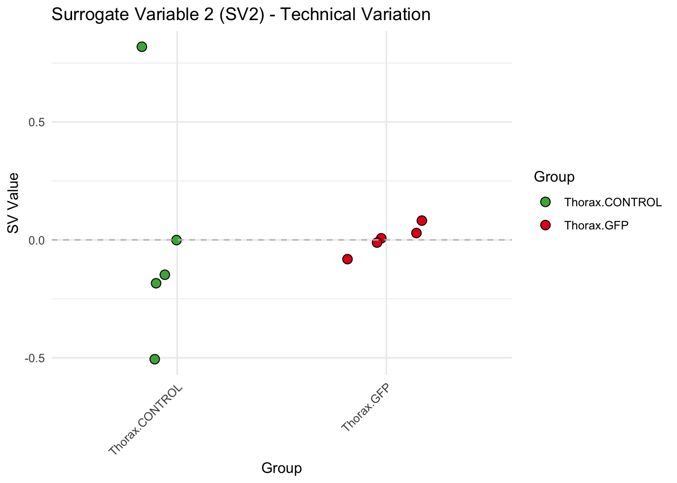
| Version | Author | Date |
|---|---|---|
| 9451c02 | Maeva TECHER | 2025-03-03 |
# Show scatter plots in the report
sva_plots$ScatterPlots[["1_2"]] # Show SV1 vs SV2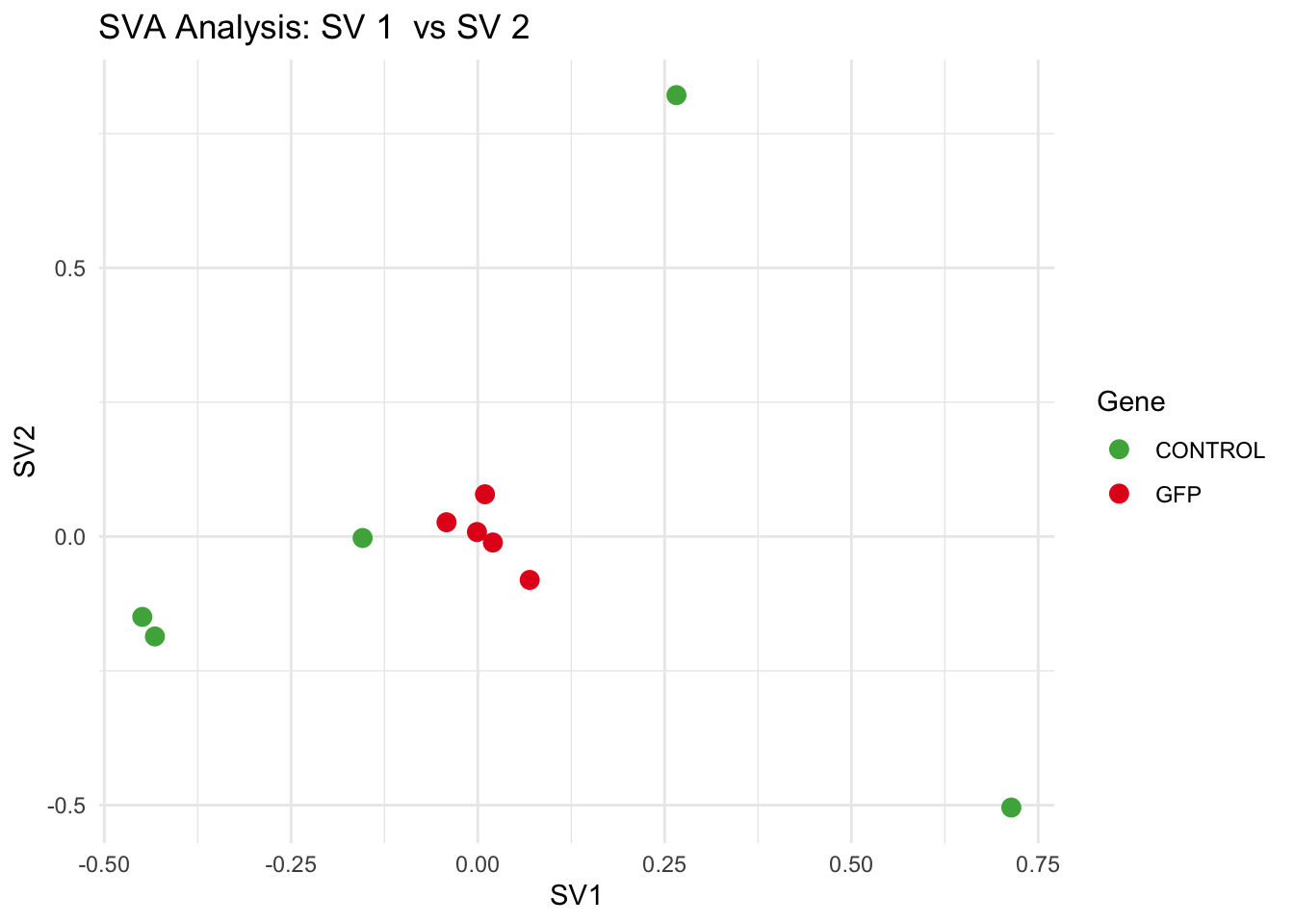
| Version | Author | Date |
|---|---|---|
| 9451c02 | Maeva TECHER | 2025-03-03 |
SV1 is clearly showing an effect of tissue. We rerun the
DESeq2 model but this time including the surrogate variable
SV2 and SV3 as a covariates only, as we know that the modeled variation
is more likely explained by tissue and gene variation rather than batch
effects.
ddssva <- dds
ddssva$SV1 <- svseq$sv[,1]
ddssva$SV2 <- svseq$sv[,2]
design(ddssva) <- ~ SV1 + SV2 + Gene
ddssva$Gene <- relevel(ddssva$Gene, ref = "CONTROL")
smallestGroupSize <- 5
keep <- rowSums(counts(ddssva) >= 10) >= smallestGroupSize
ddssva <- ddssva[keep,]
ddssva <- DESeq(ddssva)
ddssva <- ddssva[which(mcols(ddssva)$betaConv),] # remove non converging rows
### Extract results
message("Available contrasts are: ", paste(resultsNames(ddssva), collapse = ", "))
gfp <- results(ddssva, contrast = c("Gene", "GFP", "CONTROL"), alpha = 0.05)Volcano plots and Heatmaps
# Define contrast_sets
gfp_samples <- c("SGRE-THOX-CRD-1","SGRE-THOX-CRD-3","SGRE-THOX-CRD-4","SGRE-THOX-CRD-5",
"SGRE-THOX-CRD-6", "SggfpT1","SggfpT2","SggfpT3","SggfpT4","SggfpT5")
# Run full analysis
gfp_plots <- visualize_data_nopng(gfp, "GFP_vs_CONTROL", gfp_samples)
gfp_plots$volcano; gfp_plots$heatmap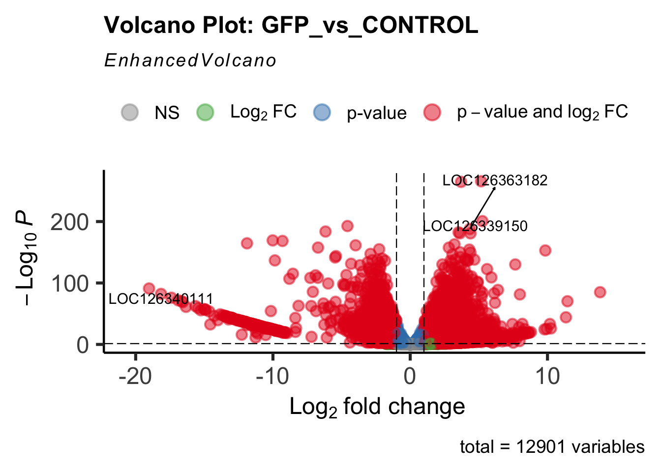
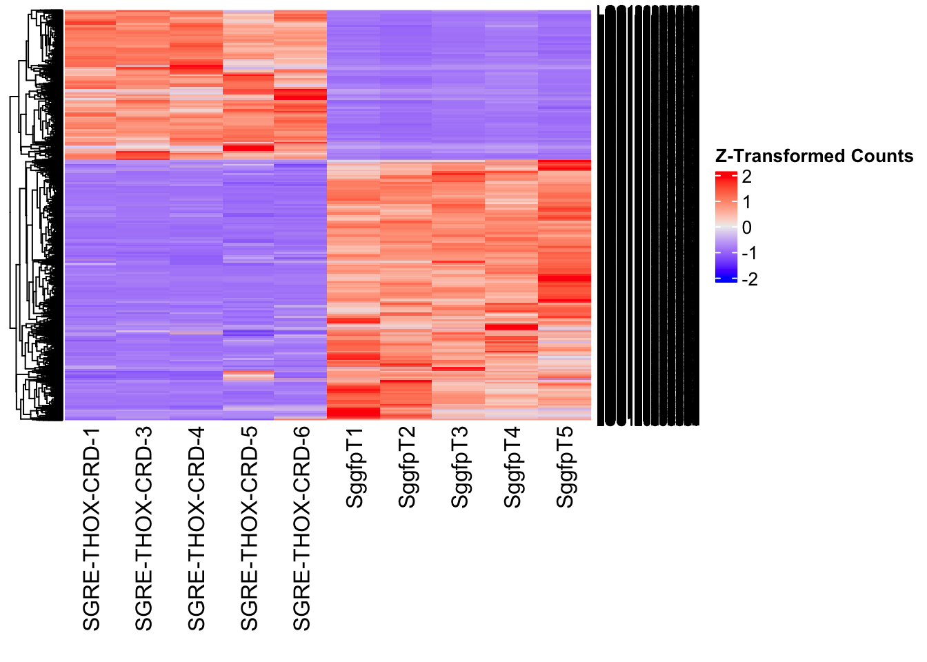
| Version | Author | Date |
|---|---|---|
| 9451c02 | Maeva TECHER | 2025-03-03 |
DEG tables
The following tables show the genes differentially expressed with at least an absolute log2fold change of > 1 considering Head tissues only. Considering GFP as the reference state, upregulated genes in knockdown treatment in red and downregulated genes in knockdown treatment in blue. You can search for a gene of interest by writting a LOCID or description in the search bar or sort by column.
# Generate tables for each contrast
table_gfp <- generate_deg_table(ddssva, "Gene_GFP_vs_CONTROL", allspecies_df)
out of 12901 with nonzero total read count
adjusted p-value < 0.05
LFC > 0 (up) : 6114, 47%
LFC < 0 (down) : 4254, 33%
outliers [1] : 0, 0%
low counts [2] : 0, 0%
(mean count < 2)
[1] see 'cooksCutoff' argument of ?results
[2] see 'independentFiltering' argument of ?resultsTotal DEGs p-value < 0.05 and absolute logFoldChange > 1: 7640LFC > 1 (up) : 4846 (63.43%)LFC < -1 (down) : 2794 (36.57%)table_gfp$kable_tableSummary and Overlap
# Summarize DEGs for all contrasts
deg_summary <- bind_rows(
summarize_deg_counts(table_gfp, "GFP vs CONTROL")
)
# Display table using kable with styling
deg_summary %>%
kable("html", escape = FALSE, col.names = gsub("_", " ", names(.))) %>%
kable_styling("striped", full_width = TRUE) %>%
column_spec(2, color = "red", bold = TRUE) %>% # Upregulated in red
column_spec(3, color = "blue", bold = TRUE) %>% # Downregulated in blue
add_header_above(c("Summary of DEGs" = 3)) %>%
row_spec(0, bold = TRUE)| Contrast | Upregulated | Downregulated |
|---|---|---|
| GFP vs CONTROL | 4834 | 2785 |
# Define the list of RNAi contrasts
contrast_list <- c("GFP_vs_CONTROL")
# Initialize empty lists for storing Head-specific DEGs for each contrast
venn_data_up <- list()
venn_data_down <- list()
venn_data_all <- list()
# Function to load Head-specific DEGs for a given set of contrasts
load_deg_contrasts_head <- function(contrast_list) {
degs_up <- list()
degs_down <- list()
degs_all <- list()
for (contrast in contrast_list) {
deg_file <- file.path(workDir, "DEG_results/RNAi/Thorax_GFP_no_rRNA/", contrast, paste0("DEG_sigresults_", contrast, ".csv"))
if (!file.exists(deg_file)) {
message(paste("File missing for contrast:", contrast))
next # Skip if the file doesn't exist
}
deg_data <- read.csv(deg_file, stringsAsFactors = FALSE)
# Convert row names to a column if necessary
if ("X" %in% colnames(deg_data)) {
colnames(deg_data)[colnames(deg_data) == "X"] <- "GeneID"
}
# Check if data is empty
if (nrow(deg_data) == 0) {
message(paste("No data for contrast:", contrast))
next
}
# Select significant DEGs (Up, Down, All)
degs_up[[contrast]] <- deg_data %>%
filter(padj < 0.05 & log2FoldChange >= 1) %>%
pull(GeneID) # Extract GeneID column
degs_down[[contrast]] <- deg_data %>%
filter(padj < 0.05 & log2FoldChange <= -1) %>%
pull(GeneID) # Extract GeneID column
degs_all[[contrast]] <- deg_data %>%
filter(padj < 0.05 & abs(log2FoldChange) >= 1) %>%
pull(GeneID) # Extract GeneID column
}
return(list(up = degs_up, down = degs_down, all = degs_all))
}
# Load DEG data for the defined contrasts (Head tissue only)
venn_data_contrasts <- load_deg_contrasts_head(contrast_list)
# Prepare the data for the Venn diagrams
venn_data_up <- venn_data_contrasts$up
venn_data_down <- venn_data_contrasts$down
venn_data_all <- venn_data_contrasts$all7. Overlap
All genes included
Head tissue
saveDir <- paste0(workDir,"/DEG_results/RNAi/Head")
# Define the RNAi contrasts of interest
rna_contrasts <- c("HEX1_vs_GFP", "HEX2_vs_GFP", "JHMT_vs_GFP", "MIOX_vs_GFP", "UNCH_vs_GFP")
# Load DEG files for each contrast
venn_data_rnai <- list()
venn_data_rnai_up <- list()
venn_data_rnai_down <- list()
for (contrast in rna_contrasts) {
deg_file <- file.path(workDir, "DEG_results/RNAi/Head", contrast, paste0("DEG_sigresults_", contrast, ".csv"))
if (!file.exists(deg_file)) {
message("File not found: ", contrast)
next
}
deg_data <- read.csv(deg_file, stringsAsFactors = FALSE)
# Rename column if needed
if ("X" %in% colnames(deg_data)) {
colnames(deg_data)[colnames(deg_data) == "X"] <- "GeneID"
}
# Store DEG sets
venn_data_rnai[[contrast]] <- deg_data %>% filter(padj < 0.05 & abs(log2FoldChange) >= 1) %>% pull(GeneID)
venn_data_rnai_up[[contrast]] <- deg_data %>% filter(padj < 0.05 & log2FoldChange >= 1) %>% pull(GeneID)
venn_data_rnai_down[[contrast]] <- deg_data %>% filter(padj < 0.05 & log2FoldChange <= -1) %>% pull(GeneID)
}
# Display Venn
display_ggvenn_plot(venn_data_rnai_up, "Venn Diagram of Head Upregulated DEGs - RNAi")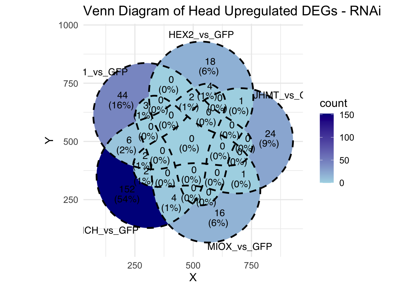
display_ggvenn_plot(venn_data_rnai_down, "Venn Diagram of Head Downregulated DEGs - RNAi")
display_ggvenn_plot(venn_data_rnai, "Venn Diagram of All Significant DEGs - RNAi")
# Display UpSet
display_upset_plot(venn_data_rnai_up, "UpSet Plot of Head Upregulated DEGs - RNAi")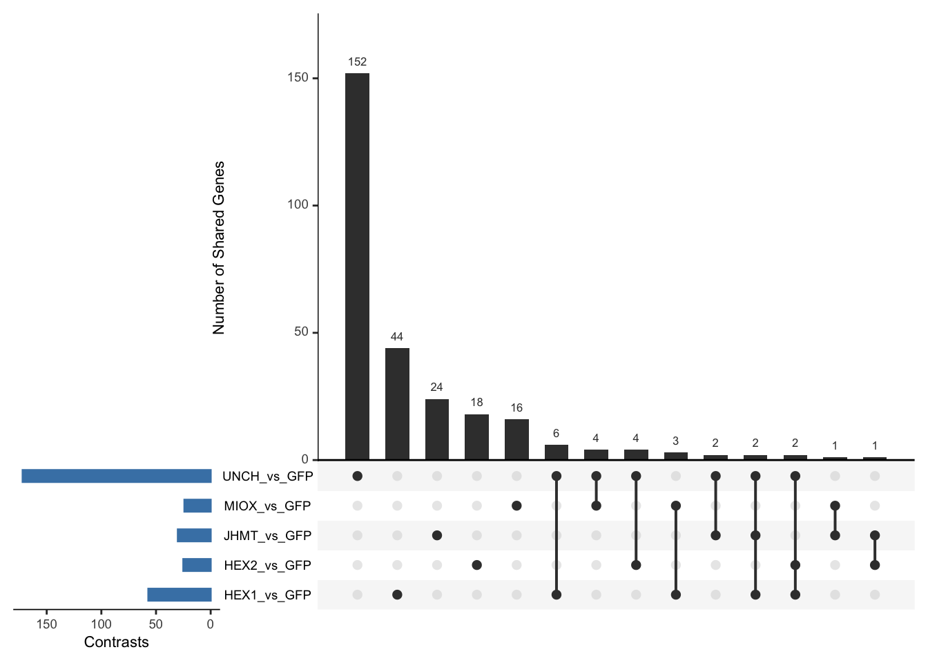
display_upset_plot(venn_data_rnai_down, "UpSet Plot of Head Downregulated DEGs - RNAi")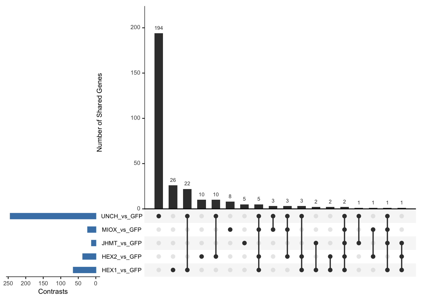
display_upset_plot(venn_data_rnai, "UpSet Plot of All Significant DEGs - RNAi")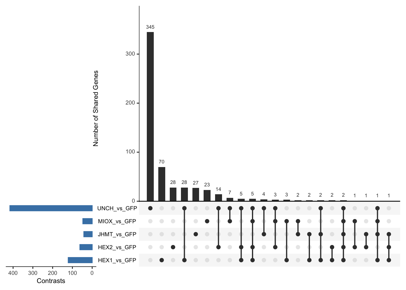
# Find intersecting GeneIDs shared by all RNAi contrasts
rna_shared_genes <- Reduce(intersect, venn_data_rnai)
# Create DataFrame for display
shared_df <- data.frame(GeneID = rna_shared_genes)
meta_shared_df <- merge(shared_df, allspecies_df, by = "GeneID", all.x = TRUE)
# Display in styled datatable
datatable(meta_shared_df, options = list(
pageLength = 10, scrollX = TRUE, autoWidth = TRUE, searchHighlight = TRUE
), rownames = FALSE) %>%
formatStyle('Species', target = 'cell', fontStyle = 'italic') %>%
formatStyle(columns = names(meta_shared_df), target = 'row',
color = styleEqual(c("red", "blue", "black"), c("red", "blue", "black")),
fontWeight = styleEqual(c("bold", "normal"), c("bold", "normal")),
backgroundColor = styleEqual(c("red", "blue", "black"), c("white", "white", "white")))# Function to extract all intersections from a named list
extract_all_upset_intersections <- function(venn_list) {
all_combinations <- unlist(lapply(1:length(venn_list), function(i) {
combn(names(venn_list), i, simplify = FALSE)
}), recursive = FALSE)
intersection_list <- list()
for (combo in all_combinations) {
combo_name <- paste(combo, collapse = " & ")
overlapping_genes <- Reduce(intersect, venn_list[combo])
if (length(overlapping_genes) > 0) {
intersection_list[[combo_name]] <- overlapping_genes
}
}
return(intersection_list)
}
# Extract all intersections for ALL DEGs
all_upset_overlaps <- extract_all_upset_intersections(venn_data_rnai)
# View names of intersections
names(all_upset_overlaps) [1] "HEX1_vs_GFP"
[2] "HEX2_vs_GFP"
[3] "JHMT_vs_GFP"
[4] "MIOX_vs_GFP"
[5] "UNCH_vs_GFP"
[6] "HEX1_vs_GFP & HEX2_vs_GFP"
[7] "HEX1_vs_GFP & JHMT_vs_GFP"
[8] "HEX1_vs_GFP & MIOX_vs_GFP"
[9] "HEX1_vs_GFP & UNCH_vs_GFP"
[10] "HEX2_vs_GFP & JHMT_vs_GFP"
[11] "HEX2_vs_GFP & MIOX_vs_GFP"
[12] "HEX2_vs_GFP & UNCH_vs_GFP"
[13] "JHMT_vs_GFP & MIOX_vs_GFP"
[14] "JHMT_vs_GFP & UNCH_vs_GFP"
[15] "MIOX_vs_GFP & UNCH_vs_GFP"
[16] "HEX1_vs_GFP & HEX2_vs_GFP & JHMT_vs_GFP"
[17] "HEX1_vs_GFP & HEX2_vs_GFP & MIOX_vs_GFP"
[18] "HEX1_vs_GFP & HEX2_vs_GFP & UNCH_vs_GFP"
[19] "HEX1_vs_GFP & JHMT_vs_GFP & MIOX_vs_GFP"
[20] "HEX1_vs_GFP & JHMT_vs_GFP & UNCH_vs_GFP"
[21] "HEX1_vs_GFP & MIOX_vs_GFP & UNCH_vs_GFP"
[22] "HEX2_vs_GFP & JHMT_vs_GFP & MIOX_vs_GFP"
[23] "HEX2_vs_GFP & JHMT_vs_GFP & UNCH_vs_GFP"
[24] "HEX2_vs_GFP & MIOX_vs_GFP & UNCH_vs_GFP"
[25] "JHMT_vs_GFP & MIOX_vs_GFP & UNCH_vs_GFP"
[26] "HEX1_vs_GFP & HEX2_vs_GFP & JHMT_vs_GFP & MIOX_vs_GFP"
[27] "HEX1_vs_GFP & HEX2_vs_GFP & JHMT_vs_GFP & UNCH_vs_GFP"
[28] "HEX1_vs_GFP & HEX2_vs_GFP & MIOX_vs_GFP & UNCH_vs_GFP"
[29] "HEX1_vs_GFP & JHMT_vs_GFP & MIOX_vs_GFP & UNCH_vs_GFP"
[30] "HEX2_vs_GFP & JHMT_vs_GFP & MIOX_vs_GFP & UNCH_vs_GFP"
[31] "HEX1_vs_GFP & HEX2_vs_GFP & JHMT_vs_GFP & MIOX_vs_GFP & UNCH_vs_GFP"# View a specific intersection
head(all_upset_overlaps[["HEX1_vs_GFP & JHMT_vs_GFP"]])[1] "LOC126300115" "LOC126316490" "LOC126318478" "LOC126306432" "LOC126320109"
[6] "LOC126318158"output_dir <- file.path(saveDir, "UpSetR_all_intersections")
dir.create(output_dir, showWarnings = FALSE)
for (name in names(all_upset_overlaps)) {
filename <- paste0(gsub(" ", "_", name), ".csv") # Replace spaces
write.csv(
data.frame(GeneID = all_upset_overlaps[[name]]),
file = file.path(output_dir, filename),
row.names = FALSE
)
}Thorax tissue
saveDir <- paste0(workDir,"/DEG_results/RNAi/Thorax")
# Define the RNAi contrasts of interest
rna_contrasts <- c("HEX1_vs_GFP", "HEX2_vs_GFP", "JHMT_vs_GFP", "MIOX_vs_GFP", "UNCH_vs_GFP")
# Load DEG files for each contrast
venn_data_rnai <- list()
venn_data_rnai_up <- list()
venn_data_rnai_down <- list()
for (contrast in rna_contrasts) {
deg_file <- file.path(workDir, "DEG_results/RNAi/Thorax", contrast, paste0("DEG_sigresults_", contrast, ".csv"))
if (!file.exists(deg_file)) {
message("File not found: ", contrast)
next
}
deg_data <- read.csv(deg_file, stringsAsFactors = FALSE)
# Rename column if needed
if ("X" %in% colnames(deg_data)) {
colnames(deg_data)[colnames(deg_data) == "X"] <- "GeneID"
}
# Store DEG sets
venn_data_rnai[[contrast]] <- deg_data %>% filter(padj < 0.05 & abs(log2FoldChange) >= 1) %>% pull(GeneID)
venn_data_rnai_up[[contrast]] <- deg_data %>% filter(padj < 0.05 & log2FoldChange >= 1) %>% pull(GeneID)
venn_data_rnai_down[[contrast]] <- deg_data %>% filter(padj < 0.05 & log2FoldChange <= -1) %>% pull(GeneID)
}
# Display Venn
display_ggvenn_plot(venn_data_rnai_up, "Venn Diagram of Thorax Upregulated DEGs - RNAi")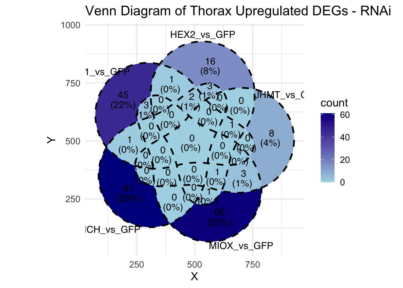
display_ggvenn_plot(venn_data_rnai_down, "Venn Diagram of Thorax Downregulated DEGs - RNAi")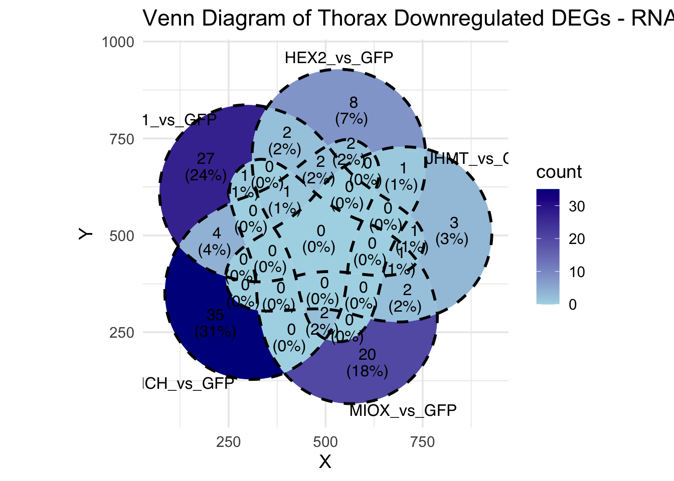
display_ggvenn_plot(venn_data_rnai, "Venn Diagram of All Significant DEGs - RNAi")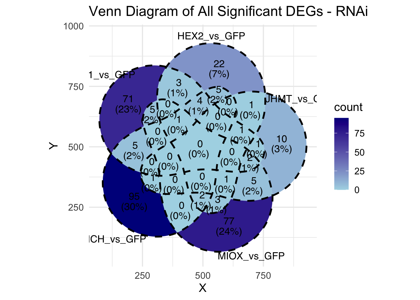
# Display UpSet
display_upset_plot(venn_data_rnai_up, "UpSet Plot of Thorax Upregulated DEGs - RNAi")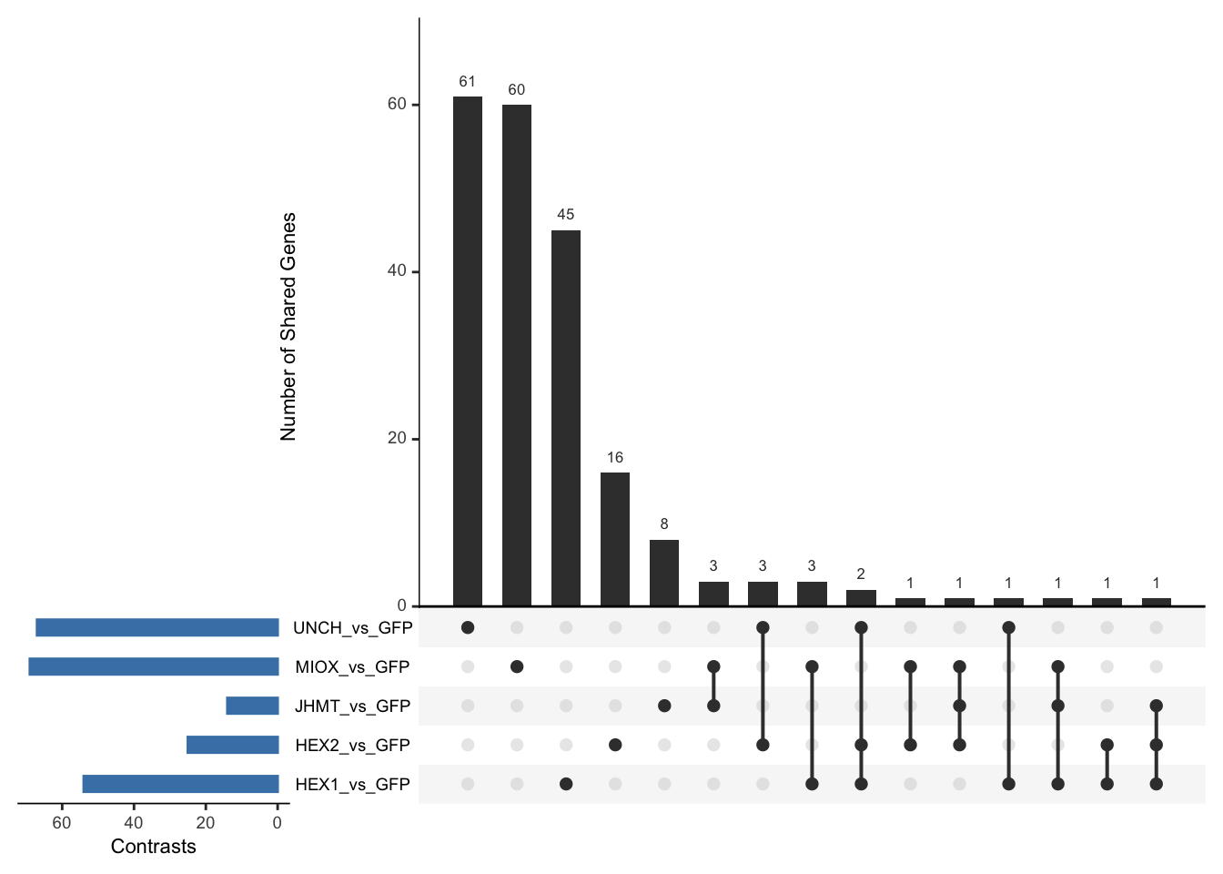
display_upset_plot(venn_data_rnai_down, "UpSet Plot of Thorax Downregulated DEGs - RNAi")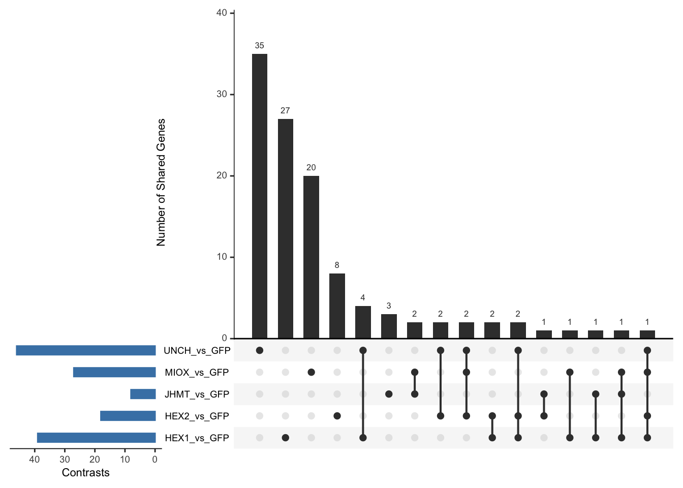
display_upset_plot(venn_data_rnai, "UpSet Plot of All Significant DEGs - RNAi")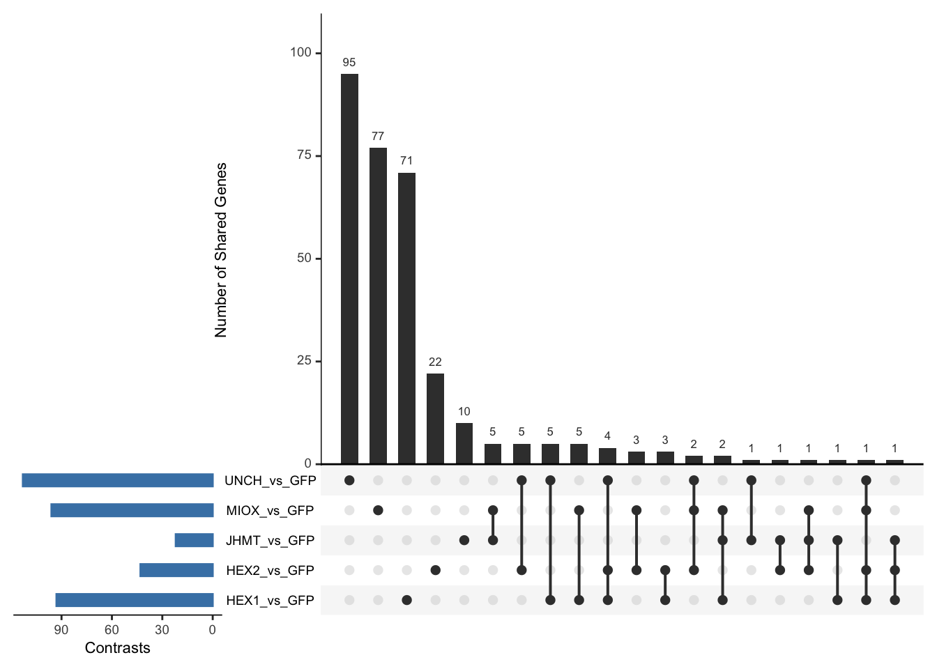
# Find intersecting GeneIDs shared by all RNAi contrasts
rna_shared_genes <- Reduce(intersect, venn_data_rnai)
# Create DataFrame for display
shared_df <- data.frame(GeneID = rna_shared_genes)
meta_shared_df <- merge(shared_df, allspecies_df, by = "GeneID", all.x = TRUE)
# Display in styled datatable
datatable(meta_shared_df, options = list(
pageLength = 10, scrollX = TRUE, autoWidth = TRUE, searchHighlight = TRUE
), rownames = FALSE) %>%
formatStyle('Species', target = 'cell', fontStyle = 'italic') %>%
formatStyle(columns = names(meta_shared_df), target = 'row',
color = styleEqual(c("red", "blue", "black"), c("red", "blue", "black")),
fontWeight = styleEqual(c("bold", "normal"), c("bold", "normal")),
backgroundColor = styleEqual(c("red", "blue", "black"), c("white", "white", "white")))# Function to extract all intersections from a named list
extract_all_upset_intersections <- function(venn_list) {
all_combinations <- unlist(lapply(1:length(venn_list), function(i) {
combn(names(venn_list), i, simplify = FALSE)
}), recursive = FALSE)
intersection_list <- list()
for (combo in all_combinations) {
combo_name <- paste(combo, collapse = " & ")
overlapping_genes <- Reduce(intersect, venn_list[combo])
if (length(overlapping_genes) > 0) {
intersection_list[[combo_name]] <- overlapping_genes
}
}
return(intersection_list)
}
# Extract all intersections for ALL DEGs
all_upset_overlaps <- extract_all_upset_intersections(venn_data_rnai)
# View names of intersections
names(all_upset_overlaps) [1] "HEX1_vs_GFP"
[2] "HEX2_vs_GFP"
[3] "JHMT_vs_GFP"
[4] "MIOX_vs_GFP"
[5] "UNCH_vs_GFP"
[6] "HEX1_vs_GFP & HEX2_vs_GFP"
[7] "HEX1_vs_GFP & JHMT_vs_GFP"
[8] "HEX1_vs_GFP & MIOX_vs_GFP"
[9] "HEX1_vs_GFP & UNCH_vs_GFP"
[10] "HEX2_vs_GFP & JHMT_vs_GFP"
[11] "HEX2_vs_GFP & MIOX_vs_GFP"
[12] "HEX2_vs_GFP & UNCH_vs_GFP"
[13] "JHMT_vs_GFP & MIOX_vs_GFP"
[14] "JHMT_vs_GFP & UNCH_vs_GFP"
[15] "MIOX_vs_GFP & UNCH_vs_GFP"
[16] "HEX1_vs_GFP & HEX2_vs_GFP & JHMT_vs_GFP"
[17] "HEX1_vs_GFP & HEX2_vs_GFP & MIOX_vs_GFP"
[18] "HEX1_vs_GFP & HEX2_vs_GFP & UNCH_vs_GFP"
[19] "HEX1_vs_GFP & JHMT_vs_GFP & MIOX_vs_GFP"
[20] "HEX1_vs_GFP & MIOX_vs_GFP & UNCH_vs_GFP"
[21] "HEX2_vs_GFP & JHMT_vs_GFP & MIOX_vs_GFP"
[22] "HEX2_vs_GFP & MIOX_vs_GFP & UNCH_vs_GFP"
[23] "HEX1_vs_GFP & HEX2_vs_GFP & MIOX_vs_GFP & UNCH_vs_GFP"# View a specific intersection
head(all_upset_overlaps[["HEX1_vs_GFP & JHMT_vs_GFP"]])[1] "LOC126337818" "LOC126321938" "LOC126318086" "LOC126319021"output_dir <- file.path(saveDir, "UpSetR_all_intersections")
dir.create(output_dir, showWarnings = FALSE)
for (name in names(all_upset_overlaps)) {
filename <- paste0(gsub(" ", "_", name), ".csv") # Replace spaces
write.csv(
data.frame(GeneID = all_upset_overlaps[[name]]),
file = file.path(output_dir, filename),
row.names = FALSE
)
}Excluding rRNA
Head tissue
saveDir <- paste0(workDir,"/DEG_results/RNAi/Head_no_rRNA")
# Define the RNAi contrasts of interest
rna_contrasts <- c("HEX1_vs_GFP", "HEX2_vs_GFP", "JHMT_vs_GFP", "MIOX_vs_GFP", "UNCH_vs_GFP")
# Load DEG files for each contrast
venn_data_rnai <- list()
venn_data_rnai_up <- list()
venn_data_rnai_down <- list()
for (contrast in rna_contrasts) {
deg_file <- file.path(workDir, "DEG_results/RNAi/Head_no_rRNA", contrast, paste0("DEG_sigresults_", contrast, ".csv"))
if (!file.exists(deg_file)) {
message("File not found: ", contrast)
next
}
deg_data <- read.csv(deg_file, stringsAsFactors = FALSE)
# Rename column if needed
if ("X" %in% colnames(deg_data)) {
colnames(deg_data)[colnames(deg_data) == "X"] <- "GeneID"
}
# Store DEG sets
venn_data_rnai[[contrast]] <- deg_data %>% filter(padj < 0.05 & abs(log2FoldChange) >= 1) %>% pull(GeneID)
venn_data_rnai_up[[contrast]] <- deg_data %>% filter(padj < 0.05 & log2FoldChange >= 1) %>% pull(GeneID)
venn_data_rnai_down[[contrast]] <- deg_data %>% filter(padj < 0.05 & log2FoldChange <= -1) %>% pull(GeneID)
}
# Display Venn
display_ggvenn_plot(venn_data_rnai_up, "Venn Diagram of Head Upregulated DEGs - RNAi")
display_ggvenn_plot(venn_data_rnai_down, "Venn Diagram of Head Downregulated DEGs - RNAi")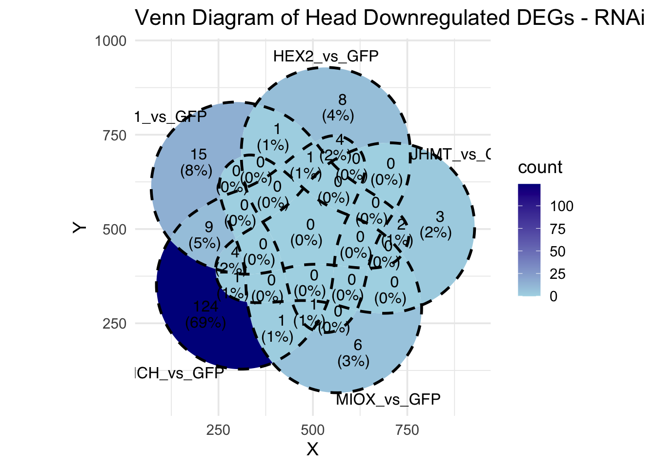
display_ggvenn_plot(venn_data_rnai, "Venn Diagram of All Significant DEGs - RNAi")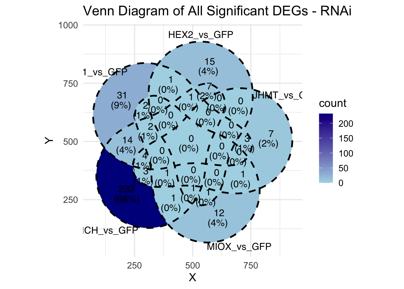
# Display UpSet
display_upset_plot(venn_data_rnai_up, "UpSet Plot of Head Upregulated DEGs - RNAi")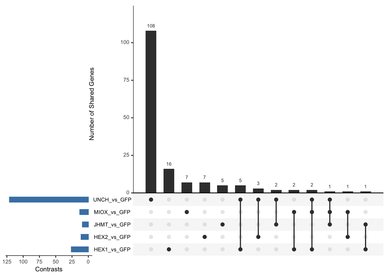
display_upset_plot(venn_data_rnai_down, "UpSet Plot of Head Downregulated DEGs - RNAi")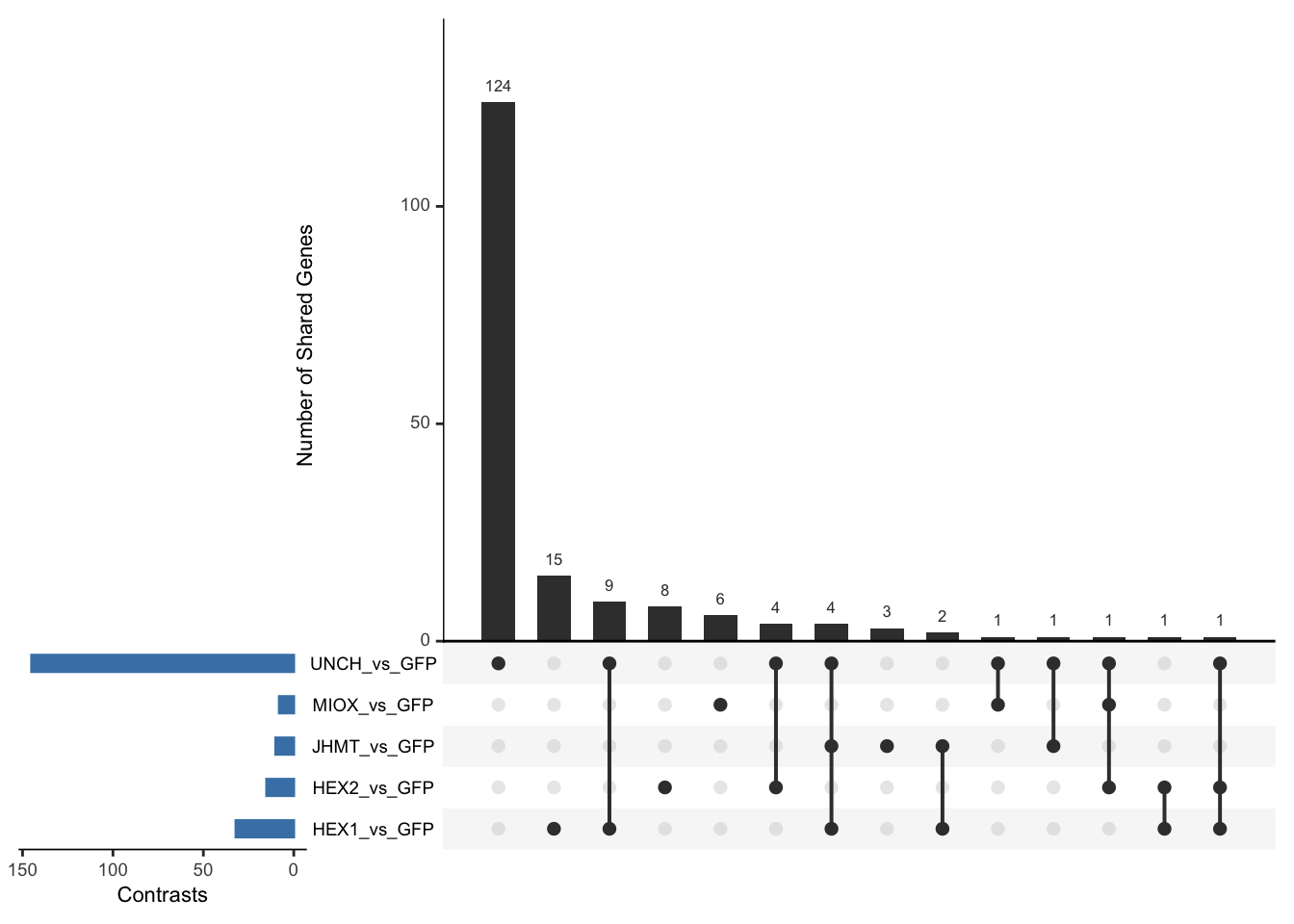
display_upset_plot(venn_data_rnai, "UpSet Plot of All Significant DEGs - RNAi")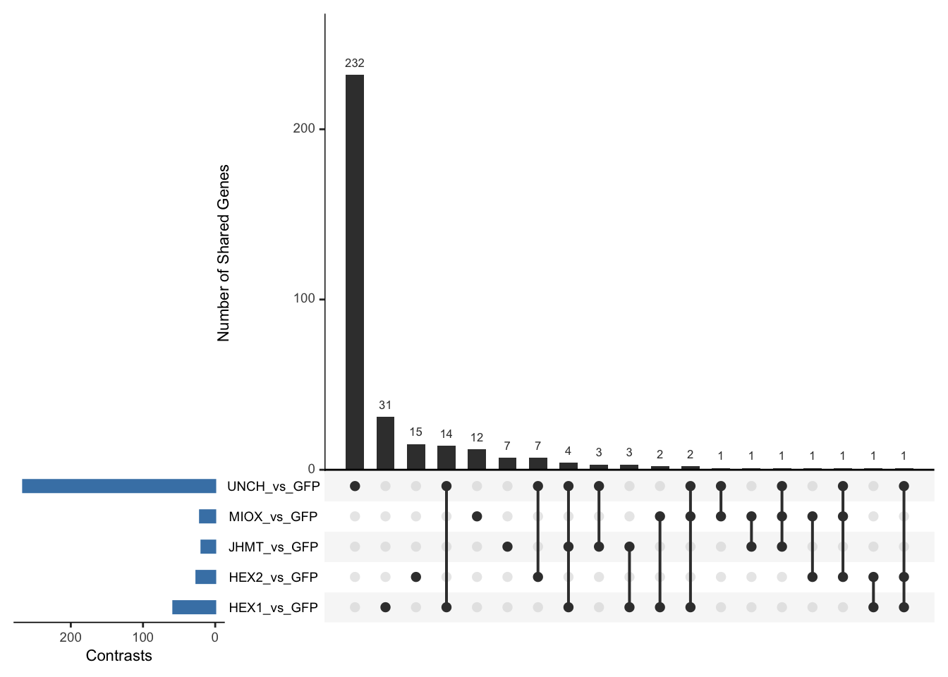
# Find intersecting GeneIDs shared by all RNAi contrasts
rna_shared_genes <- Reduce(intersect, venn_data_rnai)
# Create DataFrame for display
shared_df <- data.frame(GeneID = rna_shared_genes)
meta_shared_df <- merge(shared_df, allspecies_df, by = "GeneID", all.x = TRUE)
# Display in styled datatable
datatable(meta_shared_df, options = list(
pageLength = 10, scrollX = TRUE, autoWidth = TRUE, searchHighlight = TRUE
), rownames = FALSE) %>%
formatStyle('Species', target = 'cell', fontStyle = 'italic') %>%
formatStyle(columns = names(meta_shared_df), target = 'row',
color = styleEqual(c("red", "blue", "black"), c("red", "blue", "black")),
fontWeight = styleEqual(c("bold", "normal"), c("bold", "normal")),
backgroundColor = styleEqual(c("red", "blue", "black"), c("white", "white", "white")))# Function to extract all intersections from a named list
extract_all_upset_intersections <- function(venn_list) {
all_combinations <- unlist(lapply(1:length(venn_list), function(i) {
combn(names(venn_list), i, simplify = FALSE)
}), recursive = FALSE)
intersection_list <- list()
for (combo in all_combinations) {
combo_name <- paste(combo, collapse = " & ")
overlapping_genes <- Reduce(intersect, venn_list[combo])
if (length(overlapping_genes) > 0) {
intersection_list[[combo_name]] <- overlapping_genes
}
}
return(intersection_list)
}
# Extract all intersections for ALL DEGs
all_upset_overlaps <- extract_all_upset_intersections(venn_data_rnai)
# View names of intersections
names(all_upset_overlaps) [1] "HEX1_vs_GFP"
[2] "HEX2_vs_GFP"
[3] "JHMT_vs_GFP"
[4] "MIOX_vs_GFP"
[5] "UNCH_vs_GFP"
[6] "HEX1_vs_GFP & HEX2_vs_GFP"
[7] "HEX1_vs_GFP & JHMT_vs_GFP"
[8] "HEX1_vs_GFP & MIOX_vs_GFP"
[9] "HEX1_vs_GFP & UNCH_vs_GFP"
[10] "HEX2_vs_GFP & MIOX_vs_GFP"
[11] "HEX2_vs_GFP & UNCH_vs_GFP"
[12] "JHMT_vs_GFP & MIOX_vs_GFP"
[13] "JHMT_vs_GFP & UNCH_vs_GFP"
[14] "MIOX_vs_GFP & UNCH_vs_GFP"
[15] "HEX1_vs_GFP & HEX2_vs_GFP & UNCH_vs_GFP"
[16] "HEX1_vs_GFP & JHMT_vs_GFP & UNCH_vs_GFP"
[17] "HEX1_vs_GFP & MIOX_vs_GFP & UNCH_vs_GFP"
[18] "HEX2_vs_GFP & MIOX_vs_GFP & UNCH_vs_GFP"
[19] "JHMT_vs_GFP & MIOX_vs_GFP & UNCH_vs_GFP"# View a specific intersection
head(all_upset_overlaps[["HEX1_vs_GFP & JHMT_vs_GFP"]])[1] "LOC126285378" "LOC126356371" "LOC126336399" "LOC126284825" "LOC126355798"
[6] "LOC126306432"output_dir <- file.path(saveDir, "UpSetR_all_intersections")
dir.create(output_dir, showWarnings = FALSE)
for (name in names(all_upset_overlaps)) {
filename <- paste0(gsub(" ", "_", name), ".csv") # Replace spaces
write.csv(
data.frame(GeneID = all_upset_overlaps[[name]]),
file = file.path(output_dir, filename),
row.names = FALSE
)
}Thoax tissue
saveDir <- paste0(workDir,"/DEG_results/RNAi/Thorax_no_rRNA")
# Define the RNAi contrasts of interest
rna_contrasts <- c("HEX1_vs_GFP", "HEX2_vs_GFP", "JHMT_vs_GFP", "MIOX_vs_GFP", "UNCH_vs_GFP")
# Load DEG files for each contrast
venn_data_rnai <- list()
venn_data_rnai_up <- list()
venn_data_rnai_down <- list()
for (contrast in rna_contrasts) {
deg_file <- file.path(workDir, "DEG_results/RNAi/Thorax_no_rRNA", contrast, paste0("DEG_sigresults_", contrast, ".csv"))
if (!file.exists(deg_file)) {
message("File not found: ", contrast)
next
}
deg_data <- read.csv(deg_file, stringsAsFactors = FALSE)
# Rename column if needed
if ("X" %in% colnames(deg_data)) {
colnames(deg_data)[colnames(deg_data) == "X"] <- "GeneID"
}
# Store DEG sets
venn_data_rnai[[contrast]] <- deg_data %>% filter(padj < 0.05 & abs(log2FoldChange) >= 1) %>% pull(GeneID)
venn_data_rnai_up[[contrast]] <- deg_data %>% filter(padj < 0.05 & log2FoldChange >= 1) %>% pull(GeneID)
venn_data_rnai_down[[contrast]] <- deg_data %>% filter(padj < 0.05 & log2FoldChange <= -1) %>% pull(GeneID)
}
# Display Venn
display_ggvenn_plot(venn_data_rnai_up, "Venn Diagram of Thorax Upregulated DEGs - RNAi")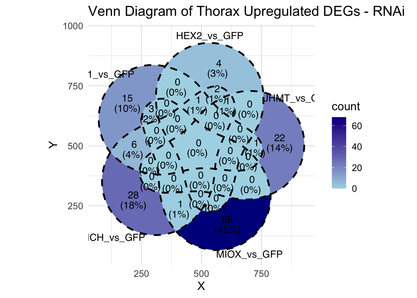
display_ggvenn_plot(venn_data_rnai_down, "Venn Diagram of Thorax Downregulated DEGs - RNAi")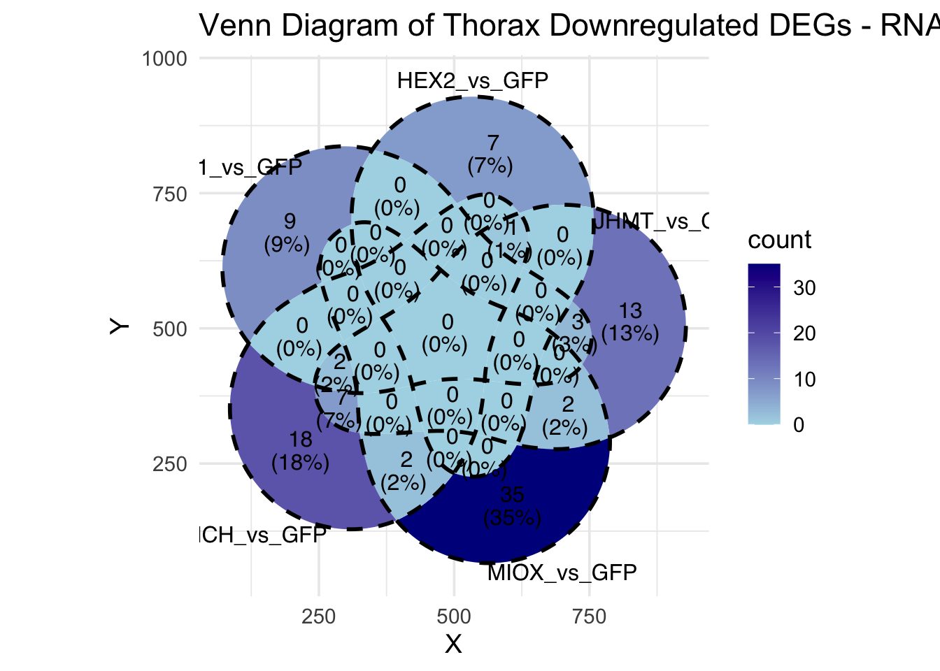
display_ggvenn_plot(venn_data_rnai, "Venn Diagram of All Significant DEGs - RNAi")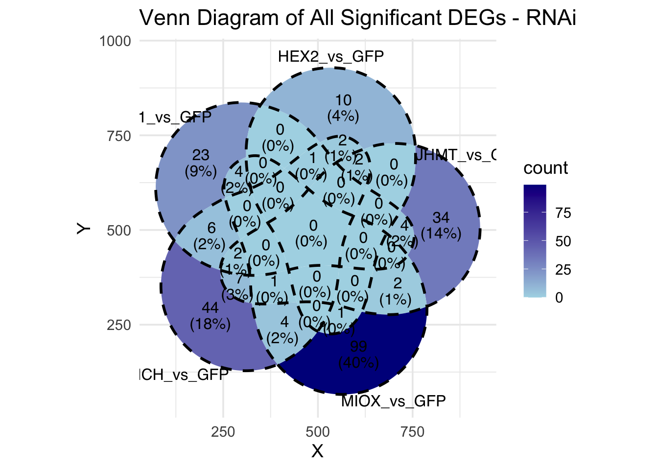
# Display UpSet
display_upset_plot(venn_data_rnai_up, "UpSet Plot of Thorax Upregulated DEGs - RNAi")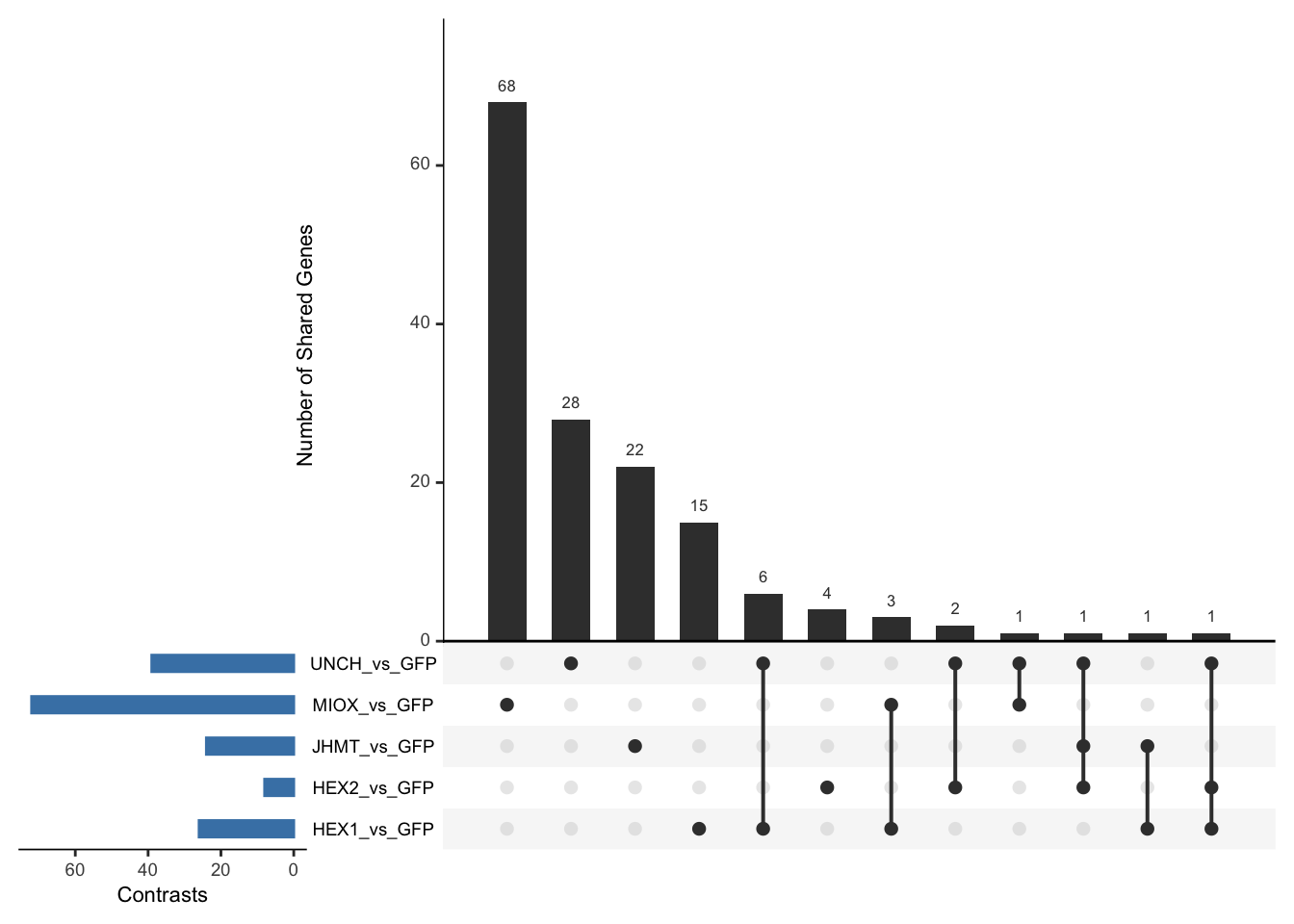
display_upset_plot(venn_data_rnai_down, "UpSet Plot of Thorax Downregulated DEGs - RNAi")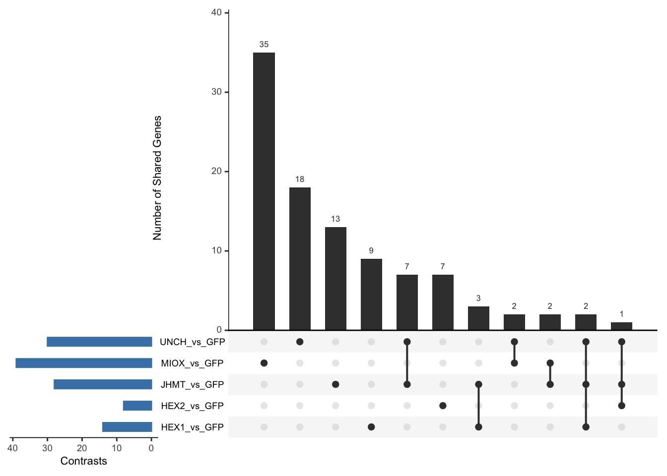
display_upset_plot(venn_data_rnai, "UpSet Plot of All Significant DEGs - RNAi")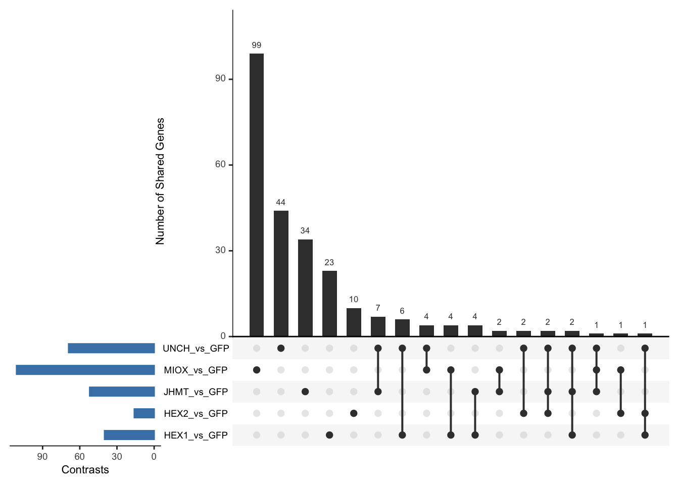
# Find intersecting GeneIDs shared by all RNAi contrasts
rna_shared_genes <- Reduce(intersect, venn_data_rnai)
# Create DataFrame for display
shared_df <- data.frame(GeneID = rna_shared_genes)
meta_shared_df <- merge(shared_df, allspecies_df, by = "GeneID", all.x = TRUE)
# Display in styled datatable
datatable(meta_shared_df, options = list(
pageLength = 10, scrollX = TRUE, autoWidth = TRUE, searchHighlight = TRUE
), rownames = FALSE) %>%
formatStyle('Species', target = 'cell', fontStyle = 'italic') %>%
formatStyle(columns = names(meta_shared_df), target = 'row',
color = styleEqual(c("red", "blue", "black"), c("red", "blue", "black")),
fontWeight = styleEqual(c("bold", "normal"), c("bold", "normal")),
backgroundColor = styleEqual(c("red", "blue", "black"), c("white", "white", "white")))# Function to extract all intersections from a named list
extract_all_upset_intersections <- function(venn_list) {
all_combinations <- unlist(lapply(1:length(venn_list), function(i) {
combn(names(venn_list), i, simplify = FALSE)
}), recursive = FALSE)
intersection_list <- list()
for (combo in all_combinations) {
combo_name <- paste(combo, collapse = " & ")
overlapping_genes <- Reduce(intersect, venn_list[combo])
if (length(overlapping_genes) > 0) {
intersection_list[[combo_name]] <- overlapping_genes
}
}
return(intersection_list)
}
# Extract all intersections for ALL DEGs
all_upset_overlaps <- extract_all_upset_intersections(venn_data_rnai)
# View names of intersections
names(all_upset_overlaps) [1] "HEX1_vs_GFP"
[2] "HEX2_vs_GFP"
[3] "JHMT_vs_GFP"
[4] "MIOX_vs_GFP"
[5] "UNCH_vs_GFP"
[6] "HEX1_vs_GFP & HEX2_vs_GFP"
[7] "HEX1_vs_GFP & JHMT_vs_GFP"
[8] "HEX1_vs_GFP & MIOX_vs_GFP"
[9] "HEX1_vs_GFP & UNCH_vs_GFP"
[10] "HEX2_vs_GFP & JHMT_vs_GFP"
[11] "HEX2_vs_GFP & MIOX_vs_GFP"
[12] "HEX2_vs_GFP & UNCH_vs_GFP"
[13] "JHMT_vs_GFP & MIOX_vs_GFP"
[14] "JHMT_vs_GFP & UNCH_vs_GFP"
[15] "MIOX_vs_GFP & UNCH_vs_GFP"
[16] "HEX1_vs_GFP & HEX2_vs_GFP & UNCH_vs_GFP"
[17] "HEX1_vs_GFP & JHMT_vs_GFP & UNCH_vs_GFP"
[18] "HEX2_vs_GFP & JHMT_vs_GFP & UNCH_vs_GFP"
[19] "JHMT_vs_GFP & MIOX_vs_GFP & UNCH_vs_GFP"# View a specific intersection
head(all_upset_overlaps[["HEX1_vs_GFP & JHMT_vs_GFP"]])[1] "LOC126285378" "LOC126336399" "LOC126336625" "LOC126355800" "LOC126354282"
[6] "LOC126272895"output_dir <- file.path(saveDir, "UpSetR_all_intersections")
dir.create(output_dir, showWarnings = FALSE)
for (name in names(all_upset_overlaps)) {
filename <- paste0(gsub(" ", "_", name), ".csv") # Replace spaces
write.csv(
data.frame(GeneID = all_upset_overlaps[[name]]),
file = file.path(output_dir, filename),
row.names = FALSE
)
}
sessionInfo()R version 4.4.2 (2024-10-31)
Platform: aarch64-apple-darwin20
Running under: macOS Sequoia 15.7.4
Matrix products: default
BLAS: /Library/Frameworks/R.framework/Versions/4.4-arm64/Resources/lib/libRblas.0.dylib
LAPACK: /Library/Frameworks/R.framework/Versions/4.4-arm64/Resources/lib/libRlapack.dylib; LAPACK version 3.12.0
locale:
[1] en_US.UTF-8/en_US.UTF-8/en_US.UTF-8/C/en_US.UTF-8/en_US.UTF-8
time zone: Asia/Tokyo
tzcode source: internal
attached base packages:
[1] grid stats4 stats graphics grDevices utils datasets
[8] methods base
other attached packages:
[1] UpSetR_1.4.0 ggVennDiagram_1.5.7
[3] VennDiagram_1.8.2 futile.logger_1.4.9
[5] tidyr_1.3.2 kableExtra_1.4.0
[7] data.table_1.18.0 DT_0.34.0
[9] rafalib_1.0.4 biomaRt_2.62.1
[11] httr2_1.2.2 purrr_1.2.1
[13] dplyr_1.1.4 ashr_2.2-63
[15] cowplot_1.2.0 sva_3.54.0
[17] BiocParallel_1.40.2 genefilter_1.88.0
[19] mgcv_1.9-4 nlme_3.1-168
[21] clusterProfiler_4.14.6 EnhancedVolcano_1.24.0
[23] circlize_0.4.17 RColorBrewer_1.1-3
[25] ComplexHeatmap_2.22.0 ensembldb_2.30.0
[27] AnnotationFilter_1.30.0 GenomicFeatures_1.58.0
[29] AnnotationHub_3.14.0 BiocFileCache_2.14.0
[31] dbplyr_2.5.1 ggConvexHull_0.1.0
[33] ggrepel_0.9.6 ggplot2_4.0.2
[35] DESeq2_1.46.0 SummarizedExperiment_1.36.0
[37] MatrixGenerics_1.18.1 matrixStats_1.5.0
[39] GenomicRanges_1.58.0 GenomeInfoDb_1.42.3
[41] org.Sgregaria.eg.db_1.0.0 AnnotationDbi_1.68.0
[43] IRanges_2.40.1 S4Vectors_0.44.0
[45] Biobase_2.66.0 BiocGenerics_0.52.0
[47] workflowr_1.7.2
loaded via a namespace (and not attached):
[1] fs_1.6.6 ProtGenerics_1.38.0 bitops_1.0-9
[4] enrichplot_1.26.6 httr_1.4.7 doParallel_1.0.17
[7] tools_4.4.2 R6_2.6.1 lazyeval_0.2.2
[10] GetoptLong_1.1.0 withr_3.0.2 gridExtra_2.3
[13] prettyunits_1.2.0 cli_3.6.5 textshaping_1.0.4
[16] formatR_1.14 Cairo_1.7-0 labeling_0.4.3
[19] sass_0.4.10 SQUAREM_2021.1 S7_0.2.1
[22] mixsqp_0.3-54 Rsamtools_2.22.0 systemfonts_1.3.1
[25] yulab.utils_0.2.3 gson_0.1.0 DOSE_4.0.1
[28] svglite_2.2.2 R.utils_2.13.0 dichromat_2.0-0.1
[31] invgamma_1.2 limma_3.62.2 rstudioapi_0.18.0
[34] RSQLite_2.4.5 generics_0.1.4 gridGraphics_0.5-1
[37] shape_1.4.6.1 BiocIO_1.16.0 crosstalk_1.2.2
[40] GO.db_3.20.0 Matrix_1.7-4 abind_1.4-8
[43] R.methodsS3_1.8.2 lifecycle_1.0.5 whisker_0.4.1
[46] yaml_2.3.12 edgeR_4.4.2 qvalue_2.38.0
[49] SparseArray_1.6.2 blob_1.3.0 promises_1.5.0
[52] crayon_1.5.3 ggtangle_0.1.1 lattice_0.22-7
[55] annotate_1.84.0 KEGGREST_1.46.0 magick_2.9.0
[58] pillar_1.11.1 knitr_1.51 fgsea_1.32.4
[61] rjson_0.2.23 codetools_0.2-20 fastmatch_1.1-8
[64] glue_1.8.0 getPass_0.2-4 ggfun_0.2.0
[67] vctrs_0.7.0 png_0.1-8 treeio_1.30.0
[70] gtable_0.3.6 cachem_1.1.0 xfun_0.56
[73] S4Arrays_1.6.0 survival_3.8-6 iterators_1.0.14
[76] statmod_1.5.1 ggtree_3.14.0 bit64_4.6.0-1
[79] progress_1.2.3 filelock_1.0.3 rprojroot_2.1.1
[82] bslib_0.9.0 irlba_2.3.5.1 otel_0.2.0
[85] colorspace_2.1-2 DBI_1.2.3 tidyselect_1.2.1
[88] processx_3.8.6 bit_4.6.0 compiler_4.4.2
[91] curl_7.0.0 git2r_0.36.2 xml2_1.5.2
[94] DelayedArray_0.32.0 rtracklayer_1.66.0 scales_1.4.0
[97] callr_3.7.6 rappdirs_0.3.4 stringr_1.6.0
[100] digest_0.6.39 rmarkdown_2.30 XVector_0.46.0
[103] htmltools_0.5.9 pkgconfig_2.0.3 fastmap_1.2.0
[106] rlang_1.1.7 GlobalOptions_0.1.3 htmlwidgets_1.6.4
[109] UCSC.utils_1.2.0 farver_2.1.2 jquerylib_0.1.4
[112] jsonlite_2.0.0 GOSemSim_2.32.0 R.oo_1.27.1
[115] RCurl_1.98-1.17 magrittr_2.0.4 GenomeInfoDbData_1.2.13
[118] ggplotify_0.1.3 patchwork_1.3.2 Rcpp_1.1.1
[121] ape_5.8-1 stringi_1.8.7 zlibbioc_1.52.0
[124] plyr_1.8.9 parallel_4.4.2 Biostrings_2.74.1
[127] splines_4.4.2 hms_1.1.4 locfit_1.5-9.12
[130] ps_1.9.1 igraph_2.2.1 reshape2_1.4.5
[133] futile.options_1.0.1 BiocVersion_3.20.0 XML_3.99-0.20
[136] evaluate_1.0.5 lambda.r_1.2.4 BiocManager_1.30.27
[139] foreach_1.5.2 httpuv_1.6.16 clue_0.3-66
[142] xtable_1.8-4 restfulr_0.0.16 tidytree_0.4.7
[145] later_1.4.5 ragg_1.5.0 viridisLite_0.4.2
[148] truncnorm_1.0-9 tibble_3.3.1 aplot_0.2.9
[151] memoise_2.0.1 GenomicAlignments_1.42.0 cluster_2.1.8.1