Signatures of selection: Did locusts or specific genes experience positive selection?
Maeva Techer
2026-04-06
Last updated: 2026-04-06
Checks: 5 2
Knit directory:
locust-comparative-genomics/
This reproducible R Markdown analysis was created with workflowr (version 1.7.2). The Checks tab describes the reproducibility checks that were applied when the results were created. The Past versions tab lists the development history.
Great! Since the R Markdown file has been committed to the Git repository, you know the exact version of the code that produced these results.
Great job! The global environment was empty. Objects defined in the global environment can affect the analysis in your R Markdown file in unknown ways. For reproduciblity it’s best to always run the code in an empty environment.
The command set.seed(20221025) was run prior to running
the code in the R Markdown file. Setting a seed ensures that any results
that rely on randomness, e.g. subsampling or permutations, are
reproducible.
Great job! Recording the operating system, R version, and package versions is critical for reproducibility.
- absrel-plot
- unnamed-chunk-21
- unnamed-chunk-27
To ensure reproducibility of the results, delete the cache directory
2_signatures-selection_cache and re-run the analysis. To
have workflowr automatically delete the cache directory prior to
building the file, set delete_cache = TRUE when running
wflow_build() or wflow_publish().
Using absolute paths to the files within your workflowr project makes it difficult for you and others to run your code on a different machine. Change the absolute path(s) below to the suggested relative path(s) to make your code more reproducible.
| absolute | relative |
|---|---|
| /Users/maevatecher/Documents/GitHub/locust-comparative-genomics/data/HYPHY_selection/combined_dnds_table.csv | data/HYPHY_selection/combined_dnds_table.csv |
| /Users/maevatecher/Documents/GitHub/locust-comparative-genomics/data/HYPHY_selection/ParsedRELAXResults/joint_busted_relax_annotated.csv | data/HYPHY_selection/ParsedRELAXResults/joint_busted_relax_annotated.csv |
| /Users/maevatecher/Documents/GitHub/locust-comparative-genomics/data/orthofinder/Polyneoptera/Results_I2_iqtree/Orthogroups/Orthogroups_SingleCopyOrthologues_selanalysiswide.txt | data/orthofinder/Polyneoptera/Results_I2_iqtree/Orthogroups/Orthogroups_SingleCopyOrthologues_selanalysiswide.txt |
| /Users/maevatecher/Documents/GitHub/locust-comparative-genomics/data/orthofinder/Polyneoptera/Results_I2_iqtree/Orthogroups/Orthogroups_CladeAssignment_WithCopyStatus_cleaned.csv | data/orthofinder/Polyneoptera/Results_I2_iqtree/Orthogroups/Orthogroups_CladeAssignment_WithCopyStatus_cleaned.csv |
| /Users/maevatecher/Documents/GitHub/locust-comparative-genomics/data/HYPHY_selection/ParsedABSRELResults_unlabeled/parsed_absrel_annotated.csv | data/HYPHY_selection/ParsedABSRELResults_unlabeled/parsed_absrel_annotated.csv |
| /Users/maevatecher/Documents/GitHub/locust-comparative-genomics/data/HYPHY_selection/ParsedABSRELResults_unlabeled/ | data/HYPHY_selection/ParsedABSRELResults_unlabeled |
| /Users/maevatecher/Documents/GitHub/locust-comparative-genomics/data/HYPHY_selection/ParsedABSRELResults_unlabeled/parsed_absrel_full.csv | data/HYPHY_selection/ParsedABSRELResults_unlabeled/parsed_absrel_full.csv |
| /Users/maevatecher/Documents/GitHub/locust-comparative-genomics/data/orthofinder/Polyneoptera/Results_I2_iqtree/Species_Tree/SpeciesTree_rooted_node_labels.txt | data/orthofinder/Polyneoptera/Results_I2_iqtree/Species_Tree/SpeciesTree_rooted_node_labels.txt |
| /Users/maevatecher/Documents/GitHub/locust-comparative-genomics/data/HYPHY_selection/ParsedABSRELResults_unlabeled/tree_colored_by_omega3_allbranches_FINAL.pdf | data/HYPHY_selection/ParsedABSRELResults_unlabeled/tree_colored_by_omega3_allbranches_FINAL.pdf |
| /Users/maevatecher/Documents/GitHub/locust-comparative-genomics/data/orthofinder/Polyneoptera/Results_I2_iqtree/trusted_ogs_v2.txt | data/orthofinder/Polyneoptera/Results_I2_iqtree/trusted_ogs_v2.txt |
| /Users/maevatecher/Documents/GitHub/locust-comparative-genomics/data/orthofinder/Polyneoptera | data/orthofinder/Polyneoptera |
| /Users/maevatecher/Documents/GitHub/locust-comparative-genomics/data | data |
| /Users/maevatecher/Documents/GitHub/locust-comparative-genomics/data/HYPHY_selection | data/HYPHY_selection |
| /Users/maevatecher/Documents/GitHub/locust-comparative-genomics/data/HYPHY_selection/ParsedBUSTEDResults_labeled/busted_results_labeled_full.csv | data/HYPHY_selection/ParsedBUSTEDResults_labeled/busted_results_labeled_full.csv |
| /Users/maevatecher/Documents/GitHub/locust-comparative-genomics/data/HYPHY_selection/ParsedBUSTEDResults_labeled_Pruned/busted_results_labeled_full.csv | data/HYPHY_selection/ParsedBUSTEDResults_labeled_Pruned/busted_results_labeled_full.csv |
| /Users/maevatecher/Documents/GitHub/locust-comparative-genomics/data/HYPHY_selection/ParsedBUSTEDResults_labeled/busted_orthogroup_summary.csv | data/HYPHY_selection/ParsedBUSTEDResults_labeled/busted_orthogroup_summary.csv |
| /Users/maevatecher/Documents/GitHub/locust-comparative-genomics/data/HYPHY_selection/ParsedRELAXResults/relax_results.csv | data/HYPHY_selection/ParsedRELAXResults/relax_results.csv |
| /Users/maevatecher/Documents/GitHub/locust-comparative-genomics/data/HYPHY_selection/ParsedRELAXResults/joint_busted_relax_results.csv | data/HYPHY_selection/ParsedRELAXResults/joint_busted_relax_results.csv |
| /Users/maevatecher/Documents/GitHub/locust-comparative-genomics/data/HYPHY_selection/ParsedBUSTEDResults_labeled_Pruned/busted_orthogroup_summary.csv | data/HYPHY_selection/ParsedBUSTEDResults_labeled_Pruned/busted_orthogroup_summary.csv |
| /Users/maevatecher/Documents/GitHub/locust-comparative-genomics/data/HYPHY_selection/ParsedRELAXResults_Pruned/relax_results.csv | data/HYPHY_selection/ParsedRELAXResults_Pruned/relax_results.csv |
| /Users/maevatecher/Documents/GitHub/locust-comparative-genomics/data/HYPHY_selection/ParsedRELAXResults_Pruned/joint_busted_relax_results.csv | data/HYPHY_selection/ParsedRELAXResults_Pruned/joint_busted_relax_results.csv |
| /Users/maevatecher/Documents/GitHub/locust-comparative-genomics/data/HYPHY_selection/ParsedRELAXResults_Pruned/joint_busted_relax_annotated.csv | data/HYPHY_selection/ParsedRELAXResults_Pruned/joint_busted_relax_annotated.csv |
Great! You are using Git for version control. Tracking code development and connecting the code version to the results is critical for reproducibility.
The results in this page were generated with repository version 34e281e. See the Past versions tab to see a history of the changes made to the R Markdown and HTML files.
Note that you need to be careful to ensure that all relevant files for
the analysis have been committed to Git prior to generating the results
(you can use wflow_publish or
wflow_git_commit). workflowr only checks the R Markdown
file, but you know if there are other scripts or data files that it
depends on. Below is the status of the Git repository when the results
were generated:
Ignored files:
    Ignored:    .DS_Store
    Ignored:    .Rhistory
    Ignored:    analysis/.DS_Store
    Ignored:    analysis/.Rhistory
    Ignored:    analysis/2_signatures-selection_cache/
    Ignored:    analysis/3_wgcna-network_cache/
    Ignored:    analysis/figure/
    Ignored:    code/.DS_Store
    Ignored:    code/scripts/.DS_Store
    Ignored:    code/scripts/pal2nal.v14/.DS_Store
    Ignored:    data/.DS_Store
    Ignored:    data/DEG_results/.DS_Store
    Ignored:    data/DEG_results/Bulk_RNAseq/.DS_Store
    Ignored:    data/DEG_results/Bulk_RNAseq/americana/.DS_Store
    Ignored:    data/DEG_results/Bulk_RNAseq/cancellata/.DS_Store
    Ignored:    data/DEG_results/Bulk_RNAseq/cubense/.DS_Store
    Ignored:    data/DEG_results/Bulk_RNAseq/gregaria/.DS_Store
    Ignored:    data/DEG_results/Bulk_RNAseq/nitens/.DS_Store
    Ignored:    data/DEG_results/RNAi/.DS_Store
    Ignored:    data/DEG_results/RNAi/All_control_no_rRNA/.DS_Store
    Ignored:    data/DEG_results/RNAi/Head/.DS_Store
    Ignored:    data/DEG_results/RNAi/Head_control/.DS_Store
    Ignored:    data/DEG_results/RNAi/Head_no_rRNA/.DS_Store
    Ignored:    data/DEG_results/RNAi/Thorax/.DS_Store
    Ignored:    data/HYPHY_selection/.DS_Store
    Ignored:    data/HYPHY_selection/ParsedABSRELResults_unlabeled/.DS_Store
    Ignored:    data/HYPHY_selection/functional_pathways/.DS_Store
    Ignored:    data/HYPHY_selection/functional_pathways/aBSREL/.DS_Store
    Ignored:    data/HYPHY_selection/pathway_enrichment/.DS_Store
    Ignored:    data/HYPHY_selection/pathway_enrichment/americana/
    Ignored:    data/HYPHY_selection/pathway_enrichment/cancellata/
    Ignored:    data/HYPHY_selection/pathway_enrichment/cubense/
    Ignored:    data/HYPHY_selection/pathway_enrichment/nitens/
    Ignored:    data/HYPHY_selection/pathway_enrichment/piceifrons/
    Ignored:    data/WGCNA/.DS_Store
    Ignored:    data/WGCNA/input/.DS_Store
    Ignored:    data/WGCNA/input/Bulk_RNAseq/.DS_Store
    Ignored:    data/WGCNA/input/GRNs/.DS_Store
    Ignored:    data/WGCNA/output/.DS_Store
    Ignored:    data/WGCNA/output/Bulk_RNAseq/.DS_Store
    Ignored:    data/WGCNA/output/Bulk_RNAseq/americana/
    Ignored:    data/WGCNA/output/Bulk_RNAseq/gregaria/.DS_Store
    Ignored:    data/WGCNA/output/Bulk_RNAseq/gregaria/Head/
    Ignored:    data/WGCNA/output/Bulk_RNAseq/gregaria/Thorax/
    Ignored:    data/behavioral_data/.DS_Store
    Ignored:    data/behavioral_data/Raw_data/.DS_Store
    Ignored:    data/cafe5_results/.DS_Store
    Ignored:    data/cafe5_results/Base_change_FILE/.DS_Store
    Ignored:    data/cafe5_results/Base_change_FILE/americana/.DS_Store
    Ignored:    data/cafe5_results/Base_change_FILE/gregaria/.DS_Store
    Ignored:    data/cafe5_results/Base_change_FILE/locusta/.DS_Store
    Ignored:    data/cafe5_results/Gene_count_FILE/.DS_Store
    Ignored:    data/list/.DS_Store
    Ignored:    data/list/Bulk_RNAseq/.DS_Store
    Ignored:    data/list/GO_Annotations/.DS_Store
    Ignored:    data/list/GO_Annotations/DesertLocustR/.DS_Store
    Ignored:    data/list/excluded_loci/.DS_Store
    Ignored:    data/orthofinder/.DS_Store
    Ignored:    data/orthofinder/Polyneoptera/.DS_Store
    Ignored:    data/orthofinder/Polyneoptera/Results_I2_iqtree/.DS_Store
    Ignored:    data/orthofinder/Polyneoptera/Results_I2_iqtree/Orthogroups/.DS_Store
    Ignored:    data/orthofinder/Polyneoptera/Results_I2_withDaust/.DS_Store
    Ignored:    data/orthofinder/Polyneoptera/Results_I2_withDaust/Orthogroups/.DS_Store
    Ignored:    data/orthofinder/Schistocerca/.DS_Store
    Ignored:    data/orthofinder/Schistocerca/Results_I2/.DS_Store
    Ignored:    data/orthofinder/Schistocerca/Results_I2/Orthogroups/.DS_Store
    Ignored:    data/overlap/.DS_Store
    Ignored:    data/pathway_enrichment/.DS_Store
    Ignored:    data/pathway_enrichment/OLD/.DS_Store
    Ignored:    data/pathway_enrichment/OLD/custom_sgregaria_orgdb/.DS_Store
    Ignored:    data/pathway_enrichment/REVIGO_results/.DS_Store
    Ignored:    data/pathway_enrichment/REVIGO_results/BP/.DS_Store
    Ignored:    data/pathway_enrichment/REVIGO_results/CC/.DS_Store
    Ignored:    data/pathway_enrichment/REVIGO_results/MF/.DS_Store
    Ignored:    data/pathway_enrichment/americana/.DS_Store
    Ignored:    data/pathway_enrichment/cancellata/.DS_Store
    Ignored:    data/pathway_enrichment/gregaria/.DS_Store
    Ignored:    data/pathway_enrichment/nitens/Thorax/
    Ignored:    data/pathway_enrichment/piceifrons/.DS_Store
    Ignored:    data/readcounts/.DS_Store
    Ignored:    data/readcounts/Bulk_RNAseq/.DS_Store
    Ignored:    data/readcounts/RNAi/.DS_Store

Untracked files:
    Untracked:  analysis/bustedPH_logomega3_scatter_nosuspect.pdf
    Untracked:  bustedPH_logomega3_scatter_nosuspect.pdf
    Untracked:  data/HYPHY_selection/functional_pathways/BUSTED_unlabeled/
    Untracked:  data/RefSeq/
    Untracked:  data/WGCNA/output/Bulk_RNAseq/cancellata/
    Untracked:  data/WGCNA/output/Bulk_RNAseq/gregaria/ModuleTraitRelationships_Head_gregaria_with_colors_name_filter.pdf
    Untracked:  data/WGCNA/output/Bulk_RNAseq/piceifrons/
    Untracked:  data/orthofinder/Polyneoptera/Results_I2_iqtree/trusted_ogs_v2.txt

Unstaged changes:
    Deleted:    analysis/2_hic-snps-phylogeny.Rmd
    Modified:   analysis/3_wgcna-network.Rmd
    Modified:   analysis/4_RNAi_behavior.Rmd
    Modified:   analysis/_site.yml
    Modified:   data/HYPHY_selection/ParsedABSRELResults_unlabeled/heatmap_significant_orthogroups.pdf
    Modified:   data/HYPHY_selection/ParsedABSRELResults_unlabeled/tree_colored_by_omega3_allbranches_FINAL.pdf
    Modified:   data/HYPHY_selection/functional_pathways/aBSREL/americana/GO_BP_dotplot_americana_aBSREL.pdf
    Modified:   data/HYPHY_selection/functional_pathways/aBSREL/americana/GO_CC_dotplot_americana_aBSREL.pdf
    Modified:   data/HYPHY_selection/functional_pathways/aBSREL/americana/GO_MF_dotplot_americana_aBSREL.pdf
    Modified:   data/HYPHY_selection/functional_pathways/aBSREL/americana/KEGG_dotplot_americana_aBSREL.pdf
    Modified:   data/HYPHY_selection/functional_pathways/aBSREL/americana/KEGG_enrichment_americana_aBSREL.csv
    Modified:   data/HYPHY_selection/functional_pathways/aBSREL/americana/enrich_KEGG_americana_aBSREL.txt
    Modified:   data/HYPHY_selection/functional_pathways/aBSREL/cancellata/GO_BP_dotplot_cancellata_aBSREL.pdf
    Modified:   data/HYPHY_selection/functional_pathways/aBSREL/cancellata/GO_CC_dotplot_cancellata_aBSREL.pdf
    Modified:   data/HYPHY_selection/functional_pathways/aBSREL/cancellata/GO_MF_dotplot_cancellata_aBSREL.pdf
    Modified:   data/HYPHY_selection/functional_pathways/aBSREL/cancellata/KEGG_dotplot_cancellata_aBSREL.pdf
    Modified:   data/HYPHY_selection/functional_pathways/aBSREL/cancellata/KEGG_enrichment_cancellata_aBSREL.csv
    Modified:   data/HYPHY_selection/functional_pathways/aBSREL/cancellata/enrich_KEGG_cancellata_aBSREL.txt
    Modified:   data/HYPHY_selection/functional_pathways/aBSREL/cubense/GO_BP_dotplot_cubense_aBSREL.pdf
    Modified:   data/HYPHY_selection/functional_pathways/aBSREL/cubense/GO_CC_dotplot_cubense_aBSREL.pdf
    Modified:   data/HYPHY_selection/functional_pathways/aBSREL/cubense/GO_MF_dotplot_cubense_aBSREL.pdf
    Modified:   data/HYPHY_selection/functional_pathways/aBSREL/cubense/KEGG_dotplot_cubense_aBSREL.pdf
    Modified:   data/HYPHY_selection/functional_pathways/aBSREL/cubense/KEGG_enrichment_cubense_aBSREL.csv
    Modified:   data/HYPHY_selection/functional_pathways/aBSREL/cubense/enrich_KEGG_cubense_aBSREL.txt
    Modified:   data/HYPHY_selection/functional_pathways/aBSREL/gregaria/GO_BP_dotplot_gregaria_aBSREL.pdf
    Modified:   data/HYPHY_selection/functional_pathways/aBSREL/gregaria/GO_CC_dotplot_gregaria_aBSREL.pdf
    Modified:   data/HYPHY_selection/functional_pathways/aBSREL/gregaria/GO_MF_dotplot_gregaria_aBSREL.pdf
    Modified:   data/HYPHY_selection/functional_pathways/aBSREL/gregaria/KEGG_dotplot_gregaria_aBSREL.pdf
    Modified:   data/HYPHY_selection/functional_pathways/aBSREL/gregaria/KEGG_enrichment_gregaria_aBSREL.csv
    Modified:   data/HYPHY_selection/functional_pathways/aBSREL/gregaria/enrich_KEGG_gregaria_aBSREL.txt
    Modified:   data/HYPHY_selection/functional_pathways/aBSREL/nitens/GO_BP_dotplot_nitens_aBSREL.pdf
    Modified:   data/HYPHY_selection/functional_pathways/aBSREL/nitens/GO_CC_dotplot_nitens_aBSREL.pdf
    Modified:   data/HYPHY_selection/functional_pathways/aBSREL/nitens/GO_MF_dotplot_nitens_aBSREL.pdf
    Modified:   data/HYPHY_selection/functional_pathways/aBSREL/nitens/KEGG_dotplot_nitens_aBSREL.pdf
    Modified:   data/HYPHY_selection/functional_pathways/aBSREL/nitens/KEGG_enrichment_nitens_aBSREL.csv
    Modified:   data/HYPHY_selection/functional_pathways/aBSREL/nitens/enrich_KEGG_nitens_aBSREL.txt
    Modified:   data/HYPHY_selection/functional_pathways/aBSREL/piceifrons/GO_BP_dotplot_piceifrons_aBSREL.pdf
    Modified:   data/HYPHY_selection/functional_pathways/aBSREL/piceifrons/GO_CC_dotplot_piceifrons_aBSREL.pdf
    Modified:   data/HYPHY_selection/functional_pathways/aBSREL/piceifrons/GO_MF_dotplot_piceifrons_aBSREL.pdf
    Modified:   data/HYPHY_selection/functional_pathways/aBSREL/piceifrons/KEGG_dotplot_piceifrons_aBSREL.pdf
    Modified:   data/HYPHY_selection/functional_pathways/aBSREL/piceifrons/KEGG_enrichment_piceifrons_aBSREL.csv
    Modified:   data/HYPHY_selection/functional_pathways/aBSREL/piceifrons/enrich_KEGG_piceifrons_aBSREL.txt
    Modified:   data/WGCNA/output/Bulk_RNAseq/gregaria/ModuleDendrogram_Head_gregaria.pdf
    Modified:   data/WGCNA/output/Bulk_RNAseq/gregaria/ModuleSizes_Head_gregaria.csv
    Modified:   data/WGCNA/output/Bulk_RNAseq/gregaria/ModuleSizes_Head_gregaria.pdf
    Modified:   data/WGCNA/output/Bulk_RNAseq/gregaria/ModuleTraitCorrelation_Head_gregaria.csv
    Modified:   data/WGCNA/output/Bulk_RNAseq/gregaria/ModuleTraitPValues_Head_gregaria.csv
    Modified:   data/WGCNA/output/Bulk_RNAseq/gregaria/ModuleTraitRelationships_Head_gregaria_with_colors.pdf
    Modified:   data/WGCNA/output/Bulk_RNAseq/gregaria/ModuleTraitRelationships_Head_gregaria_with_colors_name.pdf
    Modified:   data/WGCNA/output/Bulk_RNAseq/gregaria/SoftThreshold_Head_gregaria.pdf
    Modified:   data/WGCNA/output/Bulk_RNAseq/gregaria/network_Head_gregaria.rds
    Modified:   data/cafe5_results/Base_change_FILE/GO_BP_heatmap_top15_ExpVsCon.pdf
    Modified:   data/cafe5_results/Base_change_FILE/GO_CC_heatmap_top15_ExpVsCon.pdf
    Modified:   data/cafe5_results/Base_change_FILE/GO_MF_heatmap_top15_ExpVsCon.pdf
    Modified:   data/cafe5_results/Base_change_FILE/KEGG_subcategory_faceted_heatmap_Contraction.pdf
    Modified:   data/cafe5_results/Base_change_FILE/KEGG_subcategory_faceted_heatmap_Expansion.pdf
    Modified:   data/cafe5_results/Base_change_FILE/americana/Contraction/GO_BP_dotplot_americana_Contraction_cafe.pdf
    Modified:   data/cafe5_results/Base_change_FILE/americana/Contraction/GO_CC_dotplot_americana_Contraction_cafe.pdf
    Modified:   data/cafe5_results/Base_change_FILE/americana/Contraction/GO_MF_dotplot_americana_Contraction_cafe.pdf
    Modified:   data/cafe5_results/Base_change_FILE/americana/Contraction/KEGG_dotplot_americana_Contraction_cafe.pdf
    Modified:   data/cafe5_results/Base_change_FILE/americana/Contraction/KEGG_enrichment_americana_Contraction_cafe.csv
    Modified:   data/cafe5_results/Base_change_FILE/americana/Contraction/enrich_KEGG_americana_Contraction_cafe.txt
    Modified:   data/cafe5_results/Base_change_FILE/americana/Expansion/GO_BP_dotplot_americana_Expansion_cafe.pdf
    Modified:   data/cafe5_results/Base_change_FILE/americana/Expansion/GO_CC_dotplot_americana_Expansion_cafe.pdf
    Modified:   data/cafe5_results/Base_change_FILE/americana/Expansion/GO_MF_dotplot_americana_Expansion_cafe.pdf
    Modified:   data/cafe5_results/Base_change_FILE/americana/Expansion/KEGG_dotplot_americana_Expansion_cafe.pdf
    Modified:   data/cafe5_results/Base_change_FILE/americana/Expansion/KEGG_enrichment_americana_Expansion_cafe.csv
    Modified:   data/cafe5_results/Base_change_FILE/americana/Expansion/enrich_KEGG_americana_Expansion_cafe.txt
    Modified:   data/cafe5_results/Base_change_FILE/cancellata/Contraction/GO_BP_dotplot_cancellata_Contraction_cafe.pdf
    Modified:   data/cafe5_results/Base_change_FILE/cancellata/Contraction/GO_CC_dotplot_cancellata_Contraction_cafe.pdf
    Modified:   data/cafe5_results/Base_change_FILE/cancellata/Contraction/GO_MF_dotplot_cancellata_Contraction_cafe.pdf
    Modified:   data/cafe5_results/Base_change_FILE/cancellata/Contraction/KEGG_dotplot_cancellata_Contraction_cafe.pdf
    Modified:   data/cafe5_results/Base_change_FILE/cancellata/Contraction/KEGG_enrichment_cancellata_Contraction_cafe.csv
    Modified:   data/cafe5_results/Base_change_FILE/cancellata/Contraction/enrich_KEGG_cancellata_Contraction_cafe.txt
    Modified:   data/cafe5_results/Base_change_FILE/cancellata/Expansion/GO_BP_dotplot_cancellata_Expansion_cafe.pdf
    Modified:   data/cafe5_results/Base_change_FILE/cancellata/Expansion/GO_CC_dotplot_cancellata_Expansion_cafe.pdf
    Modified:   data/cafe5_results/Base_change_FILE/cancellata/Expansion/GO_MF_dotplot_cancellata_Expansion_cafe.pdf
    Modified:   data/cafe5_results/Base_change_FILE/cancellata/Expansion/KEGG_dotplot_cancellata_Expansion_cafe.pdf
    Modified:   data/cafe5_results/Base_change_FILE/cancellata/Expansion/KEGG_enrichment_cancellata_Expansion_cafe.csv
    Modified:   data/cafe5_results/Base_change_FILE/cancellata/Expansion/enrich_KEGG_cancellata_Expansion_cafe.txt
    Modified:   data/cafe5_results/Base_change_FILE/cubense/Contraction/GO_BP_dotplot_cubense_Contraction_cafe.pdf
    Modified:   data/cafe5_results/Base_change_FILE/cubense/Contraction/GO_CC_dotplot_cubense_Contraction_cafe.pdf
    Modified:   data/cafe5_results/Base_change_FILE/cubense/Contraction/GO_MF_dotplot_cubense_Contraction_cafe.pdf
    Modified:   data/cafe5_results/Base_change_FILE/cubense/Contraction/KEGG_dotplot_cubense_Contraction_cafe.pdf
    Modified:   data/cafe5_results/Base_change_FILE/cubense/Contraction/KEGG_enrichment_cubense_Contraction_cafe.csv
    Modified:   data/cafe5_results/Base_change_FILE/cubense/Contraction/enrich_KEGG_cubense_Contraction_cafe.txt
    Modified:   data/cafe5_results/Base_change_FILE/cubense/Expansion/GO_BP_dotplot_cubense_Expansion_cafe.pdf
    Modified:   data/cafe5_results/Base_change_FILE/cubense/Expansion/GO_CC_dotplot_cubense_Expansion_cafe.pdf
    Modified:   data/cafe5_results/Base_change_FILE/cubense/Expansion/GO_MF_dotplot_cubense_Expansion_cafe.pdf
    Modified:   data/cafe5_results/Base_change_FILE/cubense/Expansion/KEGG_dotplot_cubense_Expansion_cafe.pdf
    Modified:   data/cafe5_results/Base_change_FILE/cubense/Expansion/KEGG_enrichment_cubense_Expansion_cafe.csv
    Modified:   data/cafe5_results/Base_change_FILE/cubense/Expansion/enrich_KEGG_cubense_Expansion_cafe.txt
    Modified:   data/cafe5_results/Base_change_FILE/gregaria/Contraction/GO_BP_dotplot_gregaria_Contraction_cafe.pdf
    Modified:   data/cafe5_results/Base_change_FILE/gregaria/Contraction/GO_CC_dotplot_gregaria_Contraction_cafe.pdf
    Modified:   data/cafe5_results/Base_change_FILE/gregaria/Contraction/GO_MF_dotplot_gregaria_Contraction_cafe.pdf
    Modified:   data/cafe5_results/Base_change_FILE/gregaria/Contraction/KEGG_dotplot_gregaria_Contraction_cafe.pdf
    Modified:   data/cafe5_results/Base_change_FILE/gregaria/Contraction/KEGG_enrichment_gregaria_Contraction_cafe.csv
    Modified:   data/cafe5_results/Base_change_FILE/gregaria/Contraction/enrich_KEGG_gregaria_Contraction_cafe.txt
    Modified:   data/cafe5_results/Base_change_FILE/gregaria/Expansion/GO_BP_dotplot_gregaria_Expansion_cafe.pdf
    Modified:   data/cafe5_results/Base_change_FILE/gregaria/Expansion/GO_CC_dotplot_gregaria_Expansion_cafe.pdf
    Modified:   data/cafe5_results/Base_change_FILE/gregaria/Expansion/GO_MF_dotplot_gregaria_Expansion_cafe.pdf
    Modified:   data/cafe5_results/Base_change_FILE/gregaria/Expansion/KEGG_dotplot_gregaria_Expansion_cafe.pdf
    Modified:   data/cafe5_results/Base_change_FILE/gregaria/Expansion/KEGG_enrichment_gregaria_Expansion_cafe.csv
    Modified:   data/cafe5_results/Base_change_FILE/gregaria/Expansion/enrich_KEGG_gregaria_Expansion_cafe.txt
    Modified:   data/cafe5_results/Base_change_FILE/locusta/Contraction/GO_BP_dotplot_locusta_Contraction_cafe.pdf
    Modified:   data/cafe5_results/Base_change_FILE/locusta/Contraction/GO_CC_dotplot_locusta_Contraction_cafe.pdf
    Modified:   data/cafe5_results/Base_change_FILE/locusta/Contraction/GO_MF_dotplot_locusta_Contraction_cafe.pdf
    Modified:   data/cafe5_results/Base_change_FILE/locusta/Contraction/KEGG_dotplot_locusta_Contraction_cafe.pdf
    Modified:   data/cafe5_results/Base_change_FILE/locusta/Contraction/KEGG_enrichment_locusta_Contraction_cafe.csv
    Modified:   data/cafe5_results/Base_change_FILE/locusta/Contraction/enrich_KEGG_locusta_Contraction_cafe.txt
    Modified:   data/cafe5_results/Base_change_FILE/locusta/Expansion/GO_BP_dotplot_locusta_Expansion_cafe.pdf
    Modified:   data/cafe5_results/Base_change_FILE/locusta/Expansion/GO_CC_dotplot_locusta_Expansion_cafe.pdf
    Modified:   data/cafe5_results/Base_change_FILE/locusta/Expansion/GO_MF_dotplot_locusta_Expansion_cafe.pdf
    Modified:   data/cafe5_results/Base_change_FILE/locusta/Expansion/KEGG_dotplot_locusta_Expansion_cafe.pdf
    Modified:   data/cafe5_results/Base_change_FILE/locusta/Expansion/KEGG_enrichment_locusta_Expansion_cafe.csv
    Modified:   data/cafe5_results/Base_change_FILE/locusta/Expansion/enrich_KEGG_locusta_Expansion_cafe.txt
    Modified:   data/cafe5_results/Base_change_FILE/nitens/Contraction/GO_BP_dotplot_nitens_Contraction_cafe.pdf
    Modified:   data/cafe5_results/Base_change_FILE/nitens/Contraction/GO_CC_dotplot_nitens_Contraction_cafe.pdf
    Modified:   data/cafe5_results/Base_change_FILE/nitens/Contraction/GO_MF_dotplot_nitens_Contraction_cafe.pdf
    Modified:   data/cafe5_results/Base_change_FILE/nitens/Contraction/KEGG_dotplot_nitens_Contraction_cafe.pdf
    Modified:   data/cafe5_results/Base_change_FILE/nitens/Contraction/KEGG_enrichment_nitens_Contraction_cafe.csv
    Modified:   data/cafe5_results/Base_change_FILE/nitens/Contraction/enrich_KEGG_nitens_Contraction_cafe.txt
    Modified:   data/cafe5_results/Base_change_FILE/nitens/Expansion/GO_BP_dotplot_nitens_Expansion_cafe.pdf
    Modified:   data/cafe5_results/Base_change_FILE/nitens/Expansion/GO_CC_dotplot_nitens_Expansion_cafe.pdf
    Modified:   data/cafe5_results/Base_change_FILE/nitens/Expansion/GO_MF_dotplot_nitens_Expansion_cafe.pdf
    Modified:   data/cafe5_results/Base_change_FILE/nitens/Expansion/KEGG_dotplot_nitens_Expansion_cafe.pdf
    Modified:   data/cafe5_results/Base_change_FILE/nitens/Expansion/KEGG_enrichment_nitens_Expansion_cafe.csv
    Modified:   data/cafe5_results/Base_change_FILE/nitens/Expansion/enrich_KEGG_nitens_Expansion_cafe.txt
    Modified:   data/cafe5_results/Base_change_FILE/piceifrons/Contraction/GO_BP_dotplot_piceifrons_Contraction_cafe.pdf
    Modified:   data/cafe5_results/Base_change_FILE/piceifrons/Contraction/GO_CC_dotplot_piceifrons_Contraction_cafe.pdf
    Modified:   data/cafe5_results/Base_change_FILE/piceifrons/Contraction/GO_MF_dotplot_piceifrons_Contraction_cafe.pdf
    Modified:   data/cafe5_results/Base_change_FILE/piceifrons/Contraction/KEGG_dotplot_piceifrons_Contraction_cafe.pdf
    Modified:   data/cafe5_results/Base_change_FILE/piceifrons/Contraction/KEGG_enrichment_piceifrons_Contraction_cafe.csv
    Modified:   data/cafe5_results/Base_change_FILE/piceifrons/Contraction/enrich_KEGG_piceifrons_Contraction_cafe.txt
    Modified:   data/cafe5_results/Base_change_FILE/piceifrons/Expansion/GO_BP_dotplot_piceifrons_Expansion_cafe.pdf
    Modified:   data/cafe5_results/Base_change_FILE/piceifrons/Expansion/GO_CC_dotplot_piceifrons_Expansion_cafe.pdf
    Modified:   data/cafe5_results/Base_change_FILE/piceifrons/Expansion/GO_MF_dotplot_piceifrons_Expansion_cafe.pdf
    Modified:   data/cafe5_results/Base_change_FILE/piceifrons/Expansion/KEGG_dotplot_piceifrons_Expansion_cafe.pdf
    Modified:   data/cafe5_results/Base_change_FILE/piceifrons/Expansion/KEGG_enrichment_piceifrons_Expansion_cafe.csv
    Modified:   data/cafe5_results/Base_change_FILE/piceifrons/Expansion/enrich_KEGG_piceifrons_Expansion_cafe.txt
    Modified:   data/cafe5_results/Gene_count_FILE/GO_BP_heatmap_top15.pdf
    Modified:   data/cafe5_results/Gene_count_FILE/GO_CC_heatmap_top15.pdf
    Modified:   data/cafe5_results/Gene_count_FILE/GO_MF_heatmap_top15.pdf
    Modified:   data/cafe5_results/Gene_count_FILE/KEGG_subcategory_faceted_heatmap_Count.pdf
    Modified:   data/cafe5_results/Gene_count_FILE/americana/GO_BP_dotplot_americana_cafe.pdf
    Modified:   data/cafe5_results/Gene_count_FILE/americana/GO_CC_dotplot_americana_cafe.pdf
    Modified:   data/cafe5_results/Gene_count_FILE/americana/GO_MF_dotplot_americana_cafe.pdf
    Modified:   data/cafe5_results/Gene_count_FILE/americana/KEGG_dotplot_americana_cafe.pdf
    Modified:   data/cafe5_results/Gene_count_FILE/americana/KEGG_enrichment_americana_cafe.csv
    Modified:   data/cafe5_results/Gene_count_FILE/americana/enrich_KEGG_americana_cafe.txt
    Modified:   data/cafe5_results/Gene_count_FILE/cancellata/GO_BP_dotplot_cancellata_cafe.pdf
    Modified:   data/cafe5_results/Gene_count_FILE/cancellata/GO_CC_dotplot_cancellata_cafe.pdf
    Modified:   data/cafe5_results/Gene_count_FILE/cancellata/GO_MF_dotplot_cancellata_cafe.pdf
    Modified:   data/cafe5_results/Gene_count_FILE/cancellata/KEGG_dotplot_cancellata_cafe.pdf
    Modified:   data/cafe5_results/Gene_count_FILE/cancellata/KEGG_enrichment_cancellata_cafe.csv
    Modified:   data/cafe5_results/Gene_count_FILE/cancellata/enrich_KEGG_cancellata_cafe.txt
    Modified:   data/cafe5_results/Gene_count_FILE/cubense/GO_BP_dotplot_cubense_cafe.pdf
    Modified:   data/cafe5_results/Gene_count_FILE/cubense/GO_CC_dotplot_cubense_cafe.pdf
    Modified:   data/cafe5_results/Gene_count_FILE/cubense/GO_MF_dotplot_cubense_cafe.pdf
    Modified:   data/cafe5_results/Gene_count_FILE/cubense/KEGG_dotplot_cubense_cafe.pdf
    Modified:   data/cafe5_results/Gene_count_FILE/cubense/KEGG_enrichment_cubense_cafe.csv
    Modified:   data/cafe5_results/Gene_count_FILE/cubense/enrich_KEGG_cubense_cafe.txt
    Modified:   data/cafe5_results/Gene_count_FILE/gregaria/GO_BP_dotplot_gregaria_cafe.pdf
    Modified:   data/cafe5_results/Gene_count_FILE/gregaria/GO_CC_dotplot_gregaria_cafe.pdf
    Modified:   data/cafe5_results/Gene_count_FILE/gregaria/GO_MF_dotplot_gregaria_cafe.pdf
    Modified:   data/cafe5_results/Gene_count_FILE/gregaria/KEGG_dotplot_gregaria_cafe.pdf
    Modified:   data/cafe5_results/Gene_count_FILE/gregaria/KEGG_enrichment_gregaria_cafe.csv
    Modified:   data/cafe5_results/Gene_count_FILE/gregaria/enrich_KEGG_gregaria_cafe.txt
    Modified:   data/cafe5_results/Gene_count_FILE/locusta/GO_BP_dotplot_locusta_cafe.pdf
    Modified:   data/cafe5_results/Gene_count_FILE/locusta/GO_CC_dotplot_locusta_cafe.pdf
    Modified:   data/cafe5_results/Gene_count_FILE/locusta/GO_MF_dotplot_locusta_cafe.pdf
    Modified:   data/cafe5_results/Gene_count_FILE/locusta/KEGG_dotplot_locusta_cafe.pdf
    Modified:   data/cafe5_results/Gene_count_FILE/locusta/KEGG_enrichment_locusta_cafe.csv
    Modified:   data/cafe5_results/Gene_count_FILE/locusta/enrich_KEGG_locusta_cafe.txt
    Modified:   data/cafe5_results/Gene_count_FILE/nitens/GO_BP_dotplot_nitens_cafe.pdf
    Modified:   data/cafe5_results/Gene_count_FILE/nitens/GO_CC_dotplot_nitens_cafe.pdf
    Modified:   data/cafe5_results/Gene_count_FILE/nitens/GO_MF_dotplot_nitens_cafe.pdf
    Modified:   data/cafe5_results/Gene_count_FILE/nitens/KEGG_dotplot_nitens_cafe.pdf
    Modified:   data/cafe5_results/Gene_count_FILE/nitens/KEGG_enrichment_nitens_cafe.csv
    Modified:   data/cafe5_results/Gene_count_FILE/nitens/enrich_KEGG_nitens_cafe.txt
    Modified:   data/cafe5_results/Gene_count_FILE/piceifrons/GO_BP_dotplot_piceifrons_cafe.pdf
    Modified:   data/cafe5_results/Gene_count_FILE/piceifrons/GO_CC_dotplot_piceifrons_cafe.pdf
    Modified:   data/cafe5_results/Gene_count_FILE/piceifrons/GO_MF_dotplot_piceifrons_cafe.pdf
    Modified:   data/cafe5_results/Gene_count_FILE/piceifrons/KEGG_dotplot_piceifrons_cafe.pdf
    Modified:   data/cafe5_results/Gene_count_FILE/piceifrons/KEGG_enrichment_piceifrons_cafe.csv
    Modified:   data/cafe5_results/Gene_count_FILE/piceifrons/enrich_KEGG_piceifrons_cafe.txt
    Modified:   data/orthofinder/Polyneoptera/Results_I2_iqtree/Plots_Polyneoptera/VerticalStackedBar_A. simplex.pdf
    Modified:   data/orthofinder/Polyneoptera/Results_I2_iqtree/Plots_Polyneoptera/VerticalStackedBar_B. rossius.pdf
    Modified:   data/orthofinder/Polyneoptera/Results_I2_iqtree/Plots_Polyneoptera/VerticalStackedBar_C. secundus.pdf
    Modified:   data/orthofinder/Polyneoptera/Results_I2_iqtree/Plots_Polyneoptera/VerticalStackedBar_G. bimaculatus.pdf
    Modified:   data/orthofinder/Polyneoptera/Results_I2_iqtree/Plots_Polyneoptera/VerticalStackedBar_G. longicornis.pdf
    Modified:   data/orthofinder/Polyneoptera/Results_I2_iqtree/Plots_Polyneoptera/VerticalStackedBar_L. migratoria.pdf
    Modified:   data/orthofinder/Polyneoptera/Results_I2_iqtree/Plots_Polyneoptera/VerticalStackedBar_P. americana.pdf
    Modified:   data/orthofinder/Polyneoptera/Results_I2_iqtree/Plots_Polyneoptera/VerticalStackedBar_americana.pdf
    Modified:   data/orthofinder/Polyneoptera/Results_I2_iqtree/Plots_Polyneoptera/VerticalStackedBar_cancellata.pdf
    Modified:   data/orthofinder/Polyneoptera/Results_I2_iqtree/Plots_Polyneoptera/VerticalStackedBar_cubense.pdf
    Modified:   data/orthofinder/Polyneoptera/Results_I2_iqtree/Plots_Polyneoptera/VerticalStackedBar_gregaria.pdf
    Modified:   data/orthofinder/Polyneoptera/Results_I2_iqtree/Plots_Polyneoptera/VerticalStackedBar_nitens.pdf
    Modified:   data/orthofinder/Polyneoptera/Results_I2_iqtree/Plots_Polyneoptera/VerticalStackedBar_piceifrons.pdf
    Modified:   data/orthofinder/Schistocerca/Results_I2/Plots_Schistocerca/VerticalStackedBar_americana.pdf
    Modified:   data/orthofinder/Schistocerca/Results_I2/Plots_Schistocerca/VerticalStackedBar_cancellata.pdf
    Modified:   data/orthofinder/Schistocerca/Results_I2/Plots_Schistocerca/VerticalStackedBar_cubense.pdf
    Modified:   data/orthofinder/Schistocerca/Results_I2/Plots_Schistocerca/VerticalStackedBar_gregaria.pdf
    Modified:   data/orthofinder/Schistocerca/Results_I2/Plots_Schistocerca/VerticalStackedBar_nitens.pdf
    Modified:   data/orthofinder/Schistocerca/Results_I2/Plots_Schistocerca/VerticalStackedBar_piceifrons.pdf
Note that any generated files, e.g. HTML, png, CSS, etc., are not included in this status report because it is ok for generated content to have uncommitted changes.
These are the previous versions of the repository in which changes were
made to the R Markdown
(analysis/2_signatures-selection.Rmd) and HTML
(docs/2_signatures-selection.html) files. If you’ve
configured a remote Git repository (see ?wflow_git_remote),
click on the hyperlinks in the table below to view the files as they
were in that past version.
| File | Version | Author | Date | Message |
|---|---|---|---|---|
| html | 6e321f0 | Maeva TECHER | 2026-04-06 | Build site. |
| Rmd | 46c0324 | Maeva TECHER | 2026-04-06 | workflowr::wflow_publish("analysis/2_signatures-selection.Rmd") |
| Rmd | 3fc7f63 | Maeva TECHER | 2026-03-02 | added update last |
| html | 6075833 | Maeva TECHER | 2026-03-02 | Build site. |
| Rmd | 5e616ea | Maeva TECHER | 2026-03-02 | workflowr::wflow_publish("analysis/2_signatures-selection.Rmd") |
| Rmd | ed289b3 | Maeva TECHER | 2025-10-14 | add WGNCA |
| Rmd | d1b8eb8 | Maeva TECHER | 2025-09-17 | added last analyses |
| html | d1b8eb8 | Maeva TECHER | 2025-09-17 | added last analyses |
| Rmd | b7729ad | Maeva TECHER | 2025-09-10 | adding selction part |
| html | b7729ad | Maeva TECHER | 2025-09-10 | adding selction part |
| Rmd | 6367e32 | Maeva TECHER | 2025-09-04 | Updates PSMC |
| html | 6367e32 | Maeva TECHER | 2025-09-04 | Updates PSMC |
| html | 05239ca | Maeva TECHER | 2025-07-02 | Build site. |
| Rmd | b6a3e83 | Maeva TECHER | 2025-07-02 | workflowr::wflow_publish("analysis/2_signatures-selection.Rmd") |
| html | 6146883 | Maeva TECHER | 2025-07-01 | Build site. |
| Rmd | a2d2955 | Maeva TECHER | 2025-07-01 | Updated wgcna and compiling |
| html | a2d2955 | Maeva TECHER | 2025-07-01 | Updated wgcna and compiling |
| html | 0168e2b | Maeva TECHER | 2025-06-05 | Build site. |
| html | 9a03ca6 | Maeva TECHER | 2025-06-05 | Update website |
| html | 17484e8 | Maeva TECHER | 2025-06-05 | Build site. |
| html | 3e696d6 | Maeva TECHER | 2025-06-05 | Adding ortho heatmap |
| Rmd | 4e391c3 | Maeva TECHER | 2025-05-30 | add new analysis orthology, synteny |
| html | 4e391c3 | Maeva TECHER | 2025-05-30 | add new analysis orthology, synteny |
| Rmd | cacc1db | Maeva TECHER | 2025-05-02 | updates files |
| html | cacc1db | Maeva TECHER | 2025-05-02 | updates files |
| Rmd | b982319 | Maeva TECHER | 2025-03-03 | update font |
| html | b982319 | Maeva TECHER | 2025-03-03 | update font |
| html | f6a4762 | Maeva TECHER | 2025-02-27 | Build site. |
| Rmd | e55bac6 | Maeva TECHER | 2025-01-26 | Updating the github |
| html | e55bac6 | Maeva TECHER | 2025-01-26 | Updating the github |
| html | faf2db3 | Maeva TECHER | 2025-01-13 | update markdown |
| html | 6954b9b | Maeva TECHER | 2025-01-13 | Build site. |
| Rmd | 8df3d7c | Maeva TECHER | 2025-01-13 | changes |
| Rmd | b80db34 | Maeva TECHER | 2025-01-13 | Adding selection analysis part |
| html | b80db34 | Maeva TECHER | 2025-01-13 | Adding selection analysis part |
| html | 3fa8e62 | Maeva TECHER | 2024-11-09 | updated analysis |
| html | edb70fe | Maeva TECHER | 2024-11-08 | overlap and deg results created |
| html | ba35b82 | Maeva A. TECHER | 2024-06-20 | Build site. |
| html | acfa0db | Maeva A. TECHER | 2024-05-14 | Build site. |
| Rmd | 2c5b31c | Maeva A. TECHER | 2024-05-14 | wflow_publish("analysis/2_signatures-selection.Rmd") |
| html | 0837617 | Maeva A. TECHER | 2024-01-30 | Build site. |
| html | f701a01 | Maeva A. TECHER | 2024-01-30 | reupdate |
| html | 6e878be | Maeva A. TECHER | 2024-01-24 | Build site. |
| html | 1b09cbe | Maeva A. TECHER | 2024-01-24 | remove |
| html | 4ae7db7 | Maeva A. TECHER | 2023-12-18 | Build site. |
| Rmd | 53877fa | Maeva A. TECHER | 2023-12-18 | add pages |
Testing for signatures of selection using HyPhy: aBSREL, BUSTED and RELAX
Note: We used OrthoFinder results, PAL2NAL and HyPhy to identify signatures of selection in orthologous genes. For this part, refers to the well curated pipeline FormicidaeMolecularEvolution by Megan Barkdull (Assistant Curator of Entomology at the Natural History Museum of Los Angeles County). We describe below the modifications made and mostly copied the workflow from her Github.
We will be running three methods on our tree:
Has a gene experienced positive selection at any site in a locust species or group of species? To answer this question, we will apply BUSTED (Branch-Site Unrestricted Statistical Test for Episodic Diversification). This method works well for datasets with fewer than 10 taxa and helps identify positive selection events associated with species or groups.
Are certain species in the Schistocerca phylogeny subject to episodic (at a subset of sites) positive or purifying selection? For this analysis, we will use aBSREL (adaptive Branch-Site Random Effects Likelihood), the preferred method for detecting episodic selection on individual branches within the locust phylogeny.
Have selection pressures on genes been relaxed or intensified in a subset of Schistocerca species? For this, we will use RELAX which is not designed to detect positive selection but rather to determine whether selection pressures have been relaxed or intensified along a specified set of “test” branches.
1. Parsing orthogroups files for PAL2NAL
The script written by M. Barkdull remains unchanged; however, it
requires R with the phylotools package installed. This step
ensures that the OrthoFinder FASTA file is reordered. Instead of having
one file per orthogroup, this process consolidates the data into
species-specific files, with all orthogroups combined and properly
reordered. These files will be input for PAL2NAL, which is
a program that converts a multiple sequence alignement of proteins and
the corresponding DNA sequences (here cds) into a codon alignment.
srun --ntasks 1 --cpus-per-task 8 --mem 50G --time 04:00:00 --pty bash
ml GCC/13.2.0 OpenMPI/4.1.6 R_tamu/4.4.1 MCScanX/2024.19.19
export R_LIBS=$SCRATCH/R_LIBS_USER/
# Example for Schistocerca only
./scripts/DataMSA.R ./scripts/inputurls_Schistocerca_Jan2025.txt /scratch/group/songlab/maeva/LocustsGenomeEvolution/Schistocerca_I2/5_OrthoFinder/fasta/Results_Jan15_I2/MultipleSequenceAlignments/
# Example for Polyneoptera
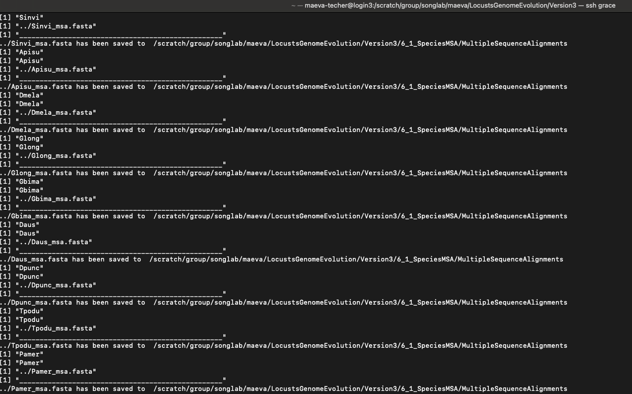
./scripts/DataMSA.R ./scripts/inputurls_13polyneoptera_May2025.txt /scratch/group/songlab/maeva/LocustsGenomeEvolution/Polyneoptera_FINAL/5_OrthoFinder/fasta/Results_May26_iqtree/MultipleSequenceAlignments/This is the final messages we get when it is successful.
Once we have obtained all the files, we go to the next step which is
filtering the protein alignment files to contain only the subset of
genes that will be called by PAL2NAL. This is due to the
fact that certain genes were not classified in orthogroups.
ml GCC/13.2.0  OpenMPI/4.1.6 R_tamu/4.4.1
export R_LIBS=$SCRATCH/R_LIBS_USER/

# Example for Schistocerca only
./scripts/FilteringCDSbyMSA.R ./scripts/inputurls_Schistocerca_Jan2025.txt

# Example for Polyneoptera
./scripts/FilteringCDSbyMSA.R ./scripts/inputurls_13polyneoptera_May2025.txt
Some of the files seems to have discrepancy of one “>” entry line
between the protein and cds file (due to a concatenation error that I
could not troubleshoot) so we are going to run the script
doublecheckCDSbyMAS which I created to remove extra
line.
# Example for Schistocerca only
./scripts/doublecheckCDSbyMAS ./scripts/inputurls_Schistocerca_Jan2025.txt

# Example for Polyneoptera
./scripts/doublecheckCDSbyMAS ./scripts/inputurls_13polyneoptera_May2025.txt

# You can also check if there is a difference with the following quick steps
grep ">" ./6_1_SpeciesMSA/proteins_Sscub.fasta | sort > proteins_Sscub_names.txt
grep ">" ./6_2_FilteredCDS/filtered_Sscub_cds.fasta | sort > cds_Sscub_names.txt
diff proteins_Sscub_names.txt cds_Sscub_names.txt
The following is the content of doublecheckCDSbyMAS:
#!/bin/bash

# Check if input file is provided
if [ "$#" -lt 1 ]; then
  echo "Usage: $0 <input_file>"
  exit 1
fi

# Input file containing species information
input_file=$1

# Directories
protein_dir="./6_1_SpeciesMSA"
cds_dir="./6_2_FilteredCDS"
backup_dir="$protein_dir/backup"
log_file="./cleaning_check.log"

# Create necessary directories
mkdir -p "$backup_dir"
rm -f "$log_file"  # Clear previous logs

# Extract species abbreviations (no header in the file)
species_list=$(awk -F',' '{print $4}' "$input_file")

# Loop through each species
for species in $species_list; do
  protein_file="$protein_dir/proteins_${species}.fasta"
  cds_file="$cds_dir/filtered_${species}_cds.fasta"
  cleaned_protein_file="$protein_dir/proteins_${species}_cleaned.fasta"
  cleaned_cds_file="$cds_dir/filtered_${species}_cds_cleaned.fasta"

  echo "Processing species: $species"

  # Check if protein and CDS files exist
  if [[ -f "$protein_file" && -f "$cds_file" ]]; then
    # Backup the original protein file
    cp "$protein_file" "$backup_dir/proteins_${species}.fasta.bak"
    echo "Backup created for: $protein_file -> $backup_dir/proteins_${species}.fasta.bak"

    # Cleaning Step: Align sequence headers between protein and CDS files
    grep ">" "$protein_file" | sort > proteins_names.txt
    grep ">" "$cds_file" | sort > cds_names.txt

    # Identify common sequence headers
    comm -12 proteins_names.txt cds_names.txt > common_names.txt

    # Check if common_names.txt is empty (indicating no matching headers)
    if [[ ! -s common_names.txt ]]; then
      echo "ERROR: No common sequence headers found for species: $species" >> "$log_file"
      echo "ERROR: Cleaning failed for species: $species due to no matching sequence headers."
      continue
    fi

    # Filter protein file
    grep -A 1 -Ff common_names.txt "$protein_file" > "$cleaned_protein_file" || {
      echo "ERROR: Failed to clean protein file for species: $species" >> "$log_file"
      continue
    }

    # Filter CDS file
    grep -A 1 -Ff common_names.txt "$cds_file" > "$cleaned_cds_file" || {
      echo "ERROR: Failed to clean CDS file for species: $species" >> "$log_file"
      continue
    }

    # Replace the original files with cleaned versions
    mv "$cleaned_protein_file" "$protein_file"
    mv "$cleaned_cds_file" "$cds_file"

    # Perform grep check to validate cleaning
    grep ">" "$protein_file" | sort > proteins_names_cleaned.txt
    grep ">" "$cds_file" | sort > cds_names_cleaned.txt
    diff_output=$(diff proteins_names_cleaned.txt cds_names_cleaned.txt)

    if [[ -z "$diff_output" ]]; then
      echo "Check passed for species: $species" >> "$log_file"
      echo "Protein and CDS sequence names match for species: $species."
    else
      echo "Check failed for species: $species" >> "$log_file"
      echo "Protein and CDS sequence names mismatch for species: $species." >> "$log_file"
      echo "$diff_output" >> "$log_file"
    fi

  else
    echo "ERROR: Missing files for species: $species" >> "$log_file"
    echo "ERROR: Protein or CDS file missing for species: $species. Skipping."
  fi
done

# Cleanup temporary files
rm -f proteins_names.txt cds_names.txt common_names.txt proteins_names_cleaned.txt cds_names_cleaned.txt

echo "All species processed. Logs saved to $log_file."
2. Generating codon-aware nucleotide alignments
PAL2NAL is installed on Grace as a module but the same
version is available in the script of this repository. We will use the
inputs generated in the previous step to obtain codon-aware
alignments.
# Example for Schistocerca only
./scripts/DataRunPAL2NAL ./scripts/inputurls_Schistocerca_Jan2025.txt

# Example for Polyneoptera
./scripts/DataRunPAL2NAL ./scripts/inputurls_13polyneoptera_May2025.txt
3. Assembling nucleotide sequence orthogroups for input in HyPHY
From M. Bardull: For some models like BUSTED, we need files that
contain orthologous nucleotide sequences from each species. Therefore,
we must recombine our codon-aware alignments in a step that is the
inverse of previous steps. To do this, use the R script
./scripts/DataSubsetCDS.R. Run with the command:
ml GCC/13.2.0  OpenMPI/4.1.6 R_tamu/4.4.1
export R_LIBS=$SCRATCH/R_LIBS_USER/

# Example for Schistocerca only
./scripts/DataSubsetCDS.R ./scripts/inputurls_Schistocerca_Jan2025.txt /scratch/group/songlab/maeva/LocustsGenomeEvolution/Schistocerca_I2/5_OrthoFinder/fasta/Results_Jan15_I2/MultipleSequenceAlignments/

# Example for Polyneoptera
 ./scripts/DataSubsetCDS.R ./scripts/inputurls_13polyneoptera_May2025.txt /scratch/group/songlab/maeva/LocustsGenomeEvolution/Polyneoptera_FINAL/5_OrthoFinder/fasta/Results_May26_iqtree/MultipleSequenceAlignments/
From M. Bardull: BUSTED will not run on sequences which contain stop
codons, even if these are reasonable, terminal stop codons.
HypPhy includes a utility which will mask these these
terminal stop codons in the orthogroups (there should be few-to-no other
stop codons, because our alignments are codon-aware). To execute this
step, use the following:
module purge
ml GCC/13.3.0  OpenMPI/5.0.3 HyPhy/2.5.71

./scripts/DataRemoveStopCodons

# for large groups launch it with sbatch
sbatch ./scripts/DataRemoveStopCodons
4. Preparing labeled phylogenies
Before performing a signature of selection analysis using HyPhy, it is important to note that some methods such as RELAX, require the phylogeny to have labeled branches to define branches. These labels define branch sets for selection testing and allow to compare selection pressures.
So we modify the script LabellingPhylogeniesHYPHY.R
ml GCC/13.2.0 OpenMPI/4.1.6 R_tamu/4.4.1
export R_LIBS=$SCRATCH/R_LIBS_USER/
# Example for Schistocerca only
./scripts/LabellingPhylogeniesHYPHY.R /scratch/group/songlab/maeva/LocustsGenomeEvolution/Schistocerca_I2/5_OrthoFinder/fasta/Results_Jan15_I2/Resolved_Gene_Trees/ Locusts.txt Locusts
# Example for Polyneoptera
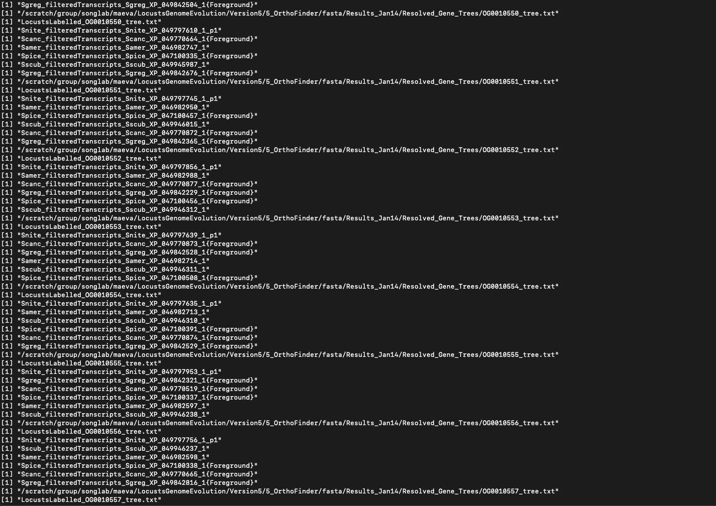
./scripts/LabellingPhylogeniesHYPHY.R /scratch/group/songlab/maeva/LocustsGenomeEvolution/Polyneoptera_FINAL/5_OrthoFinder/fasta/Results_May26_iqtree/Resolved_Gene_Trees/ Locusts.txt LocustsHow it appears when it is successful. You can see that the locust species are labelled with {Foreground}.
After running BUSTED one time, I realized that I want to check the
signal of selection only on Schistocerca and Locusta.
For that, I am pruning the trees and the fasta files of Polyneoptera if
I want to keep it with the following script
PruningLabellingPhylogeniesHYPHY.R:
ml GCC/13.2.0  OpenMPI/4.1.6 R_tamu/4.4.1
export R_LIBS=$SCRATCH/R_LIBS_USER/

  # Example for Polyneoptera
./scripts/PruningLabellingPhylogeniesHYPHY.R /scratch/group/songlab/maeva/LocustsGenomeEvolution/Polyneoptera_FINAL/5_OrthoFinder/fasta/Results_May26_iqtree/Resolved_Gene_Trees/ Locusts.txt Species2keep.txt Locusts
How the input files should look:
[maeva-techer@grace1 Polyneoptera_FINAL]$ cat Species2keep.txt
Samer
Sscub
Snite
Sgreg
Scanc
Spice
Lmigr
Details of the PruningLabellingPhylogeniesHYPHY.R are
pasted below. If we used these folders, we will have to modify our
Run{HYPHYMETHOD} to reflect the source of the new fasta sequences in
8_2_RemovedStops_Pruned:
[maeva-techer@grace1 Polyneoptera_FINAL]$ cat scripts/PruningLabellingPhylogeniesHYPHY.R
#!/usr/bin/env Rscript

# ============================= #
#        LOAD LIBRARIES        #
# ============================= #
suppressPackageStartupMessages({
  library(fs)
  library(Biostrings)
  library(ape)
  library(tidyverse)
  library(purrr)
})

# ============================= #
#         READ ARGUMENTS       #
# ============================= #
args <- commandArgs(trailingOnly = TRUE)
if (length(args) < 3) {
  stop("Usage: Rscript LabelAndPruneTreesHYPHY.R <tree_dir> <foreground_species.txt> <retained_species.txt>", call. = FALSE)
}

tree_dir <- args[1]
fg_species_file <- args[2]
retained_species_file <- args[3]
output_prefix <- ifelse(length(args) >= 4, args[4], "labelled")

# ============================= #
#       READ SPECIES FILES     #
# ============================= #
foreground_species <- read_lines(fg_species_file) %>% str_trim()
retained_species <- read_lines(retained_species_file) %>% str_trim()

# ============================= #
#         OUTPUT SETUP         #
# ============================= #
tree_output_dir <- file.path("9_1_LabelledPhylogenies_Pruned", output_prefix)
fasta_input_dir <- "8_2_RemovedStops"
fasta_output_dir <- "8_2_RemovedStops_Pruned"

dir_create(tree_output_dir)
dir_create(fasta_output_dir)

# ============================= #
#       LABEL + PRUNE FUNC     #
# ============================= #
multiTreeLabelAndPrune <- function(tree_path, retained_sp, foreground_sp, export_path) {
  tree <- read.tree(tree_path)

  message("🌳 Processing tree: ", basename(tree_path))

  # Get tip abbreviations
  tip_species <- sapply(strsplit(tree$tip.label, "_"), `[`, 1)
  keep_tips <- tree$tip.label[tip_species %in% retained_sp]

  if (length(keep_tips) < 4) {
    message("⚠️ Skipping ", basename(tree_path), " — fewer than 4 retained tips.")
    return(NULL)
  }

  pruned_tree <- drop.tip(tree, setdiff(tree$tip.label, keep_tips))

  # Label foreground tips
  pruned_tree$tip.label <- map_chr(pruned_tree$tip.label, function(label) {
    sp_abbr <- strsplit(label, "_")[[1]][1]
    if (sp_abbr %in% foreground_sp) paste0(label, "{Foreground}") else label
  })

  # Label nodes leading to foreground
  fg_tips <- grep("\\{Foreground\\}", pruned_tree$tip.label)
  if (length(fg_tips) > 0) {
    pruned_tree$node.label <- rep("", pruned_tree$Nnode)
    ancestor_nodes <- pruned_tree$edge[pruned_tree$edge[, 2] %in% fg_tips, 1]
    pruned_tree$node.label[ancestor_nodes - length(pruned_tree$tip.label)] <- "{Foreground}"
  }

  write.tree(pruned_tree, file = export_path)
  message("✅ Tree saved to: ", export_path)
}

# ============================= #
#       FASTA PRUNE FUNC       #
# ============================= #
pruneFastaBySpecies <- function(fasta_path, retained_sp, export_path) {
  message("🧬 Processing FASTA: ", basename(fasta_path))
  fasta <- readDNAStringSet(fasta_path)

  keep_idx <- vapply(names(fasta), function(x) {
    sp_abbr <- strsplit(x, "_")[[1]][1]
    sp_abbr %in% retained_sp
  }, logical(1))

  pruned_fasta <- fasta[keep_idx]
  if (length(pruned_fasta) == 0) {
    message("⚠️ No retained sequences in: ", basename(fasta_path))
    return(NULL)
  }

  writeXStringSet(pruned_fasta, filepath = export_path)
  message("✅ FASTA saved to: ", export_path)
}


# ============================= #
#         MAIN LOOP            #
# ============================= #
# Prune + label trees
tree_files <- dir_ls(tree_dir, regexp = "\\.txt$|\\.treefile$|\\.nwk$")
walk(tree_files, function(tree_file) {
  og_name <- path_file(tree_file)
  export_name <- file.path(tree_output_dir, paste0(output_prefix, "Labelled_", og_name))
  multiTreeLabelAndPrune(tree_file, retained_species, foreground_species, export_name)
})

# Prune FASTA files
fasta_files <- dir_ls(fasta_input_dir, glob = "*.fasta")
walk(fasta_files, function(fa_file) {
  out_fa <- file.path(fasta_output_dir, path_file(fa_file))
  pruneFastaBySpecies(fa_file, retained_species, out_fa)
})

message("🎉 All trees and FASTA files processed and saved.")
5. Annotating proteins with InterProScan and Orthogroups with KinFin
As part of the process, we want to make sure that the genes under selection have meaningful biological interpretations through functional annotation and GO enrichment analysis. To achieve this, we will use InterProScan to annotate individual genes and KinFin to generate gene-level annotations, assigning functional categories to entire orthogroups. This approach aligns with the orthogroup-level focus of our analyses in aBSREL, BUSTED, and RELAX, providing insights into the functional relevance of selective pressures.
For that we run the following command:
# Example for Schistocerca only
./scripts/RunningInterProScan_modif ./scripts/inputurls_Schistocerca_Jan2025.txt /scratch/group/songlab/maeva/LocustsGenomeEvolution/Schistocerca_I2/5_OrthoFinder/fasta/

# Example for Polyneoptera
./scripts/RunningInterProScan_modif ./scripts/inputurls_13polyneoptera_Jan2025.txt /scratch/group/songlab/maeva/LocustsGenomeEvolution/Polyneoptera_I2/5_OrthoFinder/fasta/

# we replace the version of interproscan to the most recent: interproscan-5.72-103.0

# we also comment out ax.set_facecolor('white')' on lines 681 and 1754 of ./kinfin/src/kinfin.py
Here is the details of
./scripts/RunningInterProScan_modif
#!/bin/bash

## SLURM Job Specifications
#SBATCH --job-name=interproscan         # Set the job name
#SBATCH --time=4-00:00:00              # Set the wall clock limit to 4 days
#SBATCH --ntasks=1                     # Request 1 task
#SBATCH --cpus-per-task=12             # Request 12 CPUs for the task
#SBATCH --mem=100G                     # Request 100GB memory
#SBATCH --output=interproscan_%j.out   # Standard output log
#SBATCH --error=interproscan_%j.err    # Standard error log

# Ensure the script receives correct arguments
if [ "$#" -ne 2 ]; then
  echo "Usage: $0 <input_file> <path_to_proteins_directory>"
  exit 1
fi

input_file=$1
proteins_dir=$2

# Load necessary modules
ml Java/11.0.2
ml WebProxy

export http_proxy=http://10.73.132.63:8080
export https_proxy=http://10.73.132.63:8080

# Main working directories
interpro_dir="./11_InterProScan/interproscan-5.72-103.0"
output_dir="$interpro_dir/out"
backup_dir="./11_InterProScan/backup"

# Create necessary directories
mkdir -p "$output_dir"
mkdir -p "$backup_dir"

# Iterate through the input file to process each species
while read -r line; do
  # Extract the species abbreviation
  name=$(echo "$line" | awk -F',' '{print $4}')
  protein_name="${name}_filteredTranscripts.fasta"

  echo "Processing species: $name"

  # Check if the protein file exists
  protein_path="$proteins_dir/$protein_name"
  if [ ! -f "$protein_path" ]; then
    echo "Protein file $protein_name not found in $proteins_dir. Skipping."
    continue
  fi

  # Check if the species has already been annotated
  annotated_file="$output_dir/${protein_name}.tsv"
  if [ -f "$annotated_file" ]; then
    echo "$annotated_file exists; skipping $name."
    continue
  fi

  # Backup original protein file and clean it
  cp "$protein_path" "$backup_dir/${protein_name}.bak"
  cp "$protein_path" "$interpro_dir/$protein_name"
  sed -i'.original' -e "s|\*||g" "$interpro_dir/$protein_name"
  rm "$interpro_dir/${protein_name}.original"

  # Run InterProScan
  echo "Running InterProScan for $protein_name..."
  cd "$interpro_dir"
  ./interproscan.sh -i "$protein_name" -d out/ -t p --goterms -appl Pfam -f TSV
  cd - > /dev/null

done < "$input_file"

# Combine all annotated results into a single file
cat "$output_dir"/*.tsv > "$interpro_dir/all_proteins.tsv"
echo "Annotation completed. Combined results stored in $interpro_dir/all_proteins.tsv."

# KinFin Preparation
kinfin_dir="./11_InterProScan/kinfin"
if [ ! -d "$kinfin_dir" ]; then
  echo "KinFin not installed. Please install KinFin and rerun this step."
  exit 1
fi

# Convert InterProScan results to KinFin-compatible format
echo "Preparing InterProScan results for KinFin..."
"$kinfin_dir/scripts/iprs2table.py" -i "$interpro_dir/all_proteins.tsv" --domain_sources Pfam

# Copy Orthofinder files to KinFin directory
cp 5_OrthoFinder/fasta/OrthoFinder/Results*/Orthogroups/Orthogroups.txt "$kinfin_dir/"
cp 5_OrthoFinder/fasta/OrthoFinder/Results*/WorkingDirectory/SequenceIDs.txt "$kinfin_dir/"
cp 5_OrthoFinder/fasta/OrthoFinder/Results*/WorkingDirectory/SpeciesIDs.txt "$kinfin_dir/"

# Create KinFin configuration file
echo '#IDX,TAXON' > "$kinfin_dir/config.txt"
sed 's/: /,/g' "$kinfin_dir/SpeciesIDs.txt" | cut -f 1 -d"." >> "$kinfin_dir/config.txt"

# Run KinFin functional annotation
echo "Running KinFin functional annotation..."
"$kinfin_dir/kinfin" --cluster_file "$kinfin_dir/Orthogroups.txt" \
  --config_file "$kinfin_dir/config.txt" \
  --sequence_ids_file "$kinfin_dir/SequenceIDs.txt" \
  --functional_annotation functional_annotation.txt

echo "Functional annotation completed."
6. dN/dS FitMG94
We will compute per gene and per branch the dN/dS score using HYPHY and the model FitMG94 as this will help us compute a mean dN/dS per branch. This analysis fits the Muse Gaut (+ GTR) model of codon substitution to an alignment and a tree and reports parameter estimates and trees scaled on expected number of synonymous and non synonymous substitutions per nucleotide site.
NB: Make sure to download the FitMG94.bf and place it in
the TemplateBatchFiles folder for HypHy otherwise it will
not work.
STEP 1. To run our analysis, we will use a loop for all orthogroups alignment and trees as follow:
#!/bin/bash

# Define paths
ALIGN_DIR="/Users/maevatecher/Desktop/Polyneoptera_FINAL/8_2_RemovedStops"
TREE_DIR="/Users/maevatecher/Desktop/Polyneoptera_FINAL/5_OrthoFinder/fasta/Results_May26_iqtree/Resolved_Gene_Trees"
HYPHY="/Users/maevatecher/miniconda3/envs/hyphy_env/bin/hyphy"
TEMPLATE="/Users/maevatecher/miniconda3/envs/hyphy_env/share/hyphy/TemplateBatchFiles/FitMG94.bf"

# Loop through all cleaned CDS alignments
for aln in ${ALIGN_DIR}/cleaned_OG*_cds.fasta; do
  # Get OG ID from filename
  og=$(basename "$aln" _cds.fasta | sed 's/^cleaned_//')

  # Define tree path and output file
  tree="${TREE_DIR}/${og}_tree.txt"
  out_json="${aln}.FITTER.json"

  # Check if tree exists
  if [[ -f "$tree" ]]; then
    echo "Running FitMG94 for $og..."
    $HYPHY "$TEMPLATE" \
      --alignment "$aln" \
      --tree "$tree" \
      --type local \
      --output "$out_json"
  else
    echo "Warning: Tree file not found for $og, skipping."
  fi
done
STEP 2. We parse the dN/dS scores computed with HyPhy in the *json file as follow:
#!/bin/bash

# Output file
output_file="combined_dnds_table.csv"

# Write header
echo "Orthogroup,Branch,Species,dN/dS" > "$output_file"

# Loop through each JSON file
for json in 8_2_RemovedStops/*.FITTER.json; do
  if [[ -f "$json" ]]; then
    # Get orthogroup name
    og=$(basename "$json" | sed 's/cleaned_//' | cut -d_ -f1)

    # Use jq to extract Branch, Species, and dN/dS
    jq -r --arg og "$og" '
      .["branch attributes"]["0"]
      | to_entries
      | map([
          $og,
          .key,
          (.key | capture("^(?<sp>[A-Z][a-z]{4})").sp // "internal"),
          .value["Confidence Intervals"].MLE
        ])
      | .[]
      | @csv
    ' "$json" >> "$output_file"
  fi
done
STEP 3. Plotting the dN/dS per Species
library(ggplot2)Warning: package 'ggplot2' was built under R version 4.4.3library(dplyr)
Attaching package: 'dplyr'The following objects are masked from 'package:stats':
filter, lagThe following objects are masked from 'package:base':
intersect, setdiff, setequal, unionlibrary(readr)Warning: package 'readr' was built under R version 4.4.3library(broom)Warning: package 'broom' was built under R version 4.4.3library(tidyr)Warning: package 'tidyr' was built under R version 4.4.3# Load data
dnds_data <- read_csv("/Users/maevatecher/Documents/GitHub/locust-comparative-genomics/data/HYPHY_selection/combined_dnds_table.csv")Rows: 309886 Columns: 4── Column specification ────────────────────────────────────────────────────────
Delimiter: ","
chr (3): Orthogroup, Branch, Species
dbl (1): dN/dS
ℹ Use `spec()` to retrieve the full column specification for this data.
ℹ Specify the column types or set `show_col_types = FALSE` to quiet this message.colnames(dnds_data)[colnames(dnds_data) == "Orthogroup"] <- "orthogroup"
relax_data <- read_csv("/Users/maevatecher/Documents/GitHub/locust-comparative-genomics/data/HYPHY_selection/ParsedRELAXResults/joint_busted_relax_annotated.csv")Rows: 5339 Columns: 53
── Column specification ────────────────────────────────────────────────────────
Delimiter: ","
chr (11): orthogroup, selection_status, file, input_file, selection_type, As...
dbl (39): pval_foreground, padj_foreground, pval_background, padj_background...
lgl (3): suspect_result.x, suspect_result.y, significant
ℹ Use `spec()` to retrieve the full column specification for this data.
ℹ Specify the column types or set `show_col_types = FALSE` to quiet this message.# Load the list of orthogroups (one per line)
single_copy_OGs <- read_lines("/Users/maevatecher/Documents/GitHub/locust-comparative-genomics/data/orthofinder/Polyneoptera/Results_I2_iqtree/Orthogroups/Orthogroups_SingleCopyOrthologues_selanalysiswide.txt")
# Extract PSG
psg_df <- relax_data %>%
dplyr::select(orthogroup, selection_status, suspect_result.x) %>%
filter(suspect_result.x == "FALSE") %>%
mutate(PSG = selection_status %in% c("Foreground only", "Both foreground and background")) %>%
distinct()
# Merge and clean
dnds_data <- dnds_data %>%
left_join(psg_df, by = "orthogroup") %>%
mutate(
PSG = ifelse(is.na(PSG), FALSE, PSG),
Species = factor(Species, levels = c("Lmigr", "Sgreg", "Scanc", "Spice", "Samer", "Sscub", "Snite")),
`dN/dS` = as.numeric(`dN/dS`),
locust_group = ifelse(Species %in% c("Lmigr", "Sgreg", "Scanc", "Spice"), "Locust", "Other")
) %>%
filter(!is.na(`dN/dS`), !is.na(Species), `dN/dS` <= 1) %>%
filter(orthogroup %in% single_copy_OGs)
# PLOT
ggplot(dnds_data, aes(x = Species, y = `dN/dS`, fill = locust_group)) +
geom_violin(
aes(group = Species),
scale = "area",
trim = FALSE,
adjust = 1.2,
alpha = 0.7,
color = "black"
) +
# geom_jitter(
# aes(color = PSG),
# width = 0.15,
# size = 0.8,
# alpha = 0.5
# ) +
# Add red mean lines
stat_summary(
fun = mean,
geom = "crossbar",
width = 0.3,
color = "red",
fatten = 3
) +
facet_wrap(
~ PSG,
labeller = labeller(PSG = c(`TRUE` = "PSG Orthogroups", `FALSE` = "Non-PSG Orthogroups"))
) +
scale_fill_manual(values = c("Locust" = "gray60", "Other" = "white")) +
scale_color_manual(values = c("TRUE" = "#D95F02", "FALSE" = "gray80")) +
coord_cartesian(ylim = c(0, 1)) +
labs(
title = "Raincloud Violin Plot of dN/dS per Species",
subtitle = "Faceted by PSG Status; Locusts shaded in gray; Red line = mean",
x = "Species",
y = "dN/dS"
) +
theme_minimal(base_size = 14) +
theme(
strip.text = element_text(face = "bold"),
axis.text.x = element_text(angle = 45, hjust = 1)
)Warning: The `fatten` argument of `geom_crossbar()` is deprecated as of ggplot2 4.0.0.
ℹ Please use the `middle.linewidth` argument instead.
This warning is displayed once per session.
Call `lifecycle::last_lifecycle_warnings()` to see where this warning was
generated.Warning: No shared levels found between `names(values)` of the manual scale and the
data's colour values.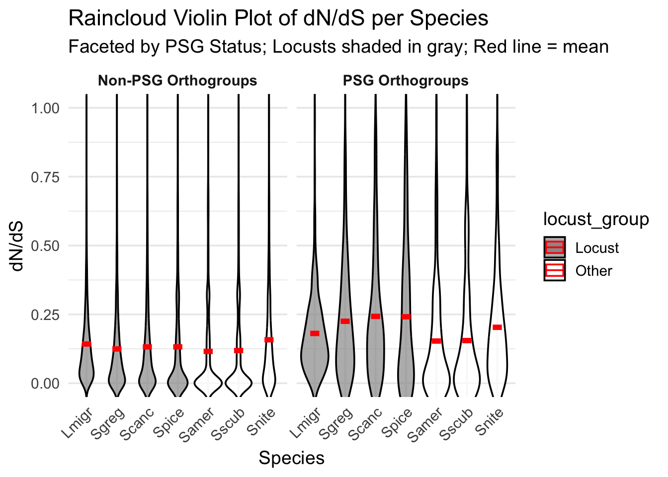
ggplot(dnds_data, aes(x = Species, y = `dN/dS`, fill = PSG)) +
geom_violin(
aes(group = interaction(Species, PSG)),
position = position_dodge(width = 0.6), # smaller = less gap
scale = "width",
width = 0.7, # narrower violins
trim = FALSE,
adjust = 1.2,
alpha = 0.7,
color = "black"
) +
stat_summary(
aes(group = PSG),
fun = mean,
geom = "crossbar",
width = 0.2,
color = "red",
fatten = 3,
position = position_dodge(width = 0.6)
) +
scale_fill_manual(values = c(`TRUE` = "#D95F02", `FALSE` = "gray70"),
labels = c(`TRUE` = "PSG", `FALSE` = "Non-PSG")) +
coord_cartesian(ylim = c(0, 1)) +
labs(
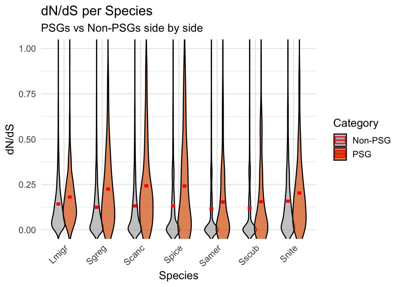
title = "dN/dS per Species",
subtitle = "PSGs vs Non-PSGs side by side",
x = "Species",
y = "dN/dS",
fill = "Category"
) +
theme_minimal(base_size = 14) +
theme(
axis.text.x = element_text(angle = 45, hjust = 1)
)
We are adding statistical test using a Wilcoxon tests between PSG and non-PSG per species:
library(broom)
library(dplyr)
library(tidyr)

# -----------------------------
# Wilcoxon test per species
# -----------------------------
stat_test_results <- dnds_data %>%
  group_by(Species) %>%
  summarise(
    n_psg = sum(PSG == TRUE, na.rm = TRUE),
    n_nonpsg = sum(PSG == FALSE, na.rm = TRUE),
    p_value = if (n_psg > 0 && n_nonpsg > 0) {
      wilcox.test(`dN/dS` ~ PSG)$p.value
    } else {
      NA_real_
    },
    .groups = "drop"
  ) %>%
  mutate(
    p_adj = p.adjust(p_value, method = "fdr")
  )

print(stat_test_results)
# A tibble: 7 × 5
Species n_psg n_nonpsg p_value p_adj
<fct> <int> <int> <dbl> <dbl>
1 Lmigr 378 4282 6.56e-13 1.15e-12
2 Sgreg 412 4839 1.87e-30 6.54e-30
3 Scanc 411 4757 7.03e-31 4.92e-30
4 Spice 385 4626 1.20e-18 2.79e-18
5 Samer 382 4479 1.57e- 6 1.83e- 6
6 Sscub 383 4515 3.89e- 5 3.89e- 5
7 Snite 414 4707 1.22e- 9 1.71e- 9# -----------------------------
# ANOVA + Tukey, corrected
# -----------------------------
# Make a copy so we do not disturb the plotting object if you want to keep PSG logical there
# Make a copy for ANOVA/Tukey
dnds_aov <- dnds_data %>%
mutate(
PSG_factor = factor(PSG, levels = c(FALSE, TRUE), labels = c("NonPSG", "PSG")),
Group = interaction(Species, PSG_factor, sep = "_")
)
# ANOVA
aov_model <- aov(`dN/dS` ~ Group, data = dnds_aov)
summary(aov_model) Df Sum Sq Mean Sq F value Pr(>F)
Group 13 21.4 1.6472 48.19 <2e-16 ***
Residuals 34956 1194.7 0.0342
---
Signif. codes: 0 '***' 0.001 '**' 0.01 '*' 0.05 '.' 0.1 ' ' 1# Tukey
tukey_res <- TukeyHSD(aov_model, which = "Group")
# install if needed
if (!requireNamespace("multcompView", quietly = TRUE)) install.packages("multcompView")
library(multcompView)
# Extract Tukey results
tukey_df <- as.data.frame(tukey_res$Group)
tukey_df$Comparison <- rownames(tukey_df)
# Named p-values
pvals <- tukey_df$`p adj`
names(pvals) <- tukey_df$Comparison
# Compact letter display
group_letters <- multcompView::multcompLetters(pvals)$Letters
# Convert back to dataframe
group_df <- data.frame(
Group = names(group_letters),
Letters = group_letters
) %>%
tidyr::separate(Group, into = c("Species", "PSG"), sep = "_", remove = FALSE)
print(group_df) Group Species PSG Letters
Sgreg_NonPSG Sgreg_NonPSG Sgreg NonPSG ab
Scanc_NonPSG Scanc_NonPSG Scanc NonPSG ac
Spice_NonPSG Spice_NonPSG Spice NonPSG ac
Samer_NonPSG Samer_NonPSG Samer NonPSG b
Sscub_NonPSG Sscub_NonPSG Sscub NonPSG b
Snite_NonPSG Snite_NonPSG Snite NonPSG d
Lmigr_PSG Lmigr_PSG Lmigr PSG de
Sgreg_PSG Sgreg_PSG Sgreg PSG f
Scanc_PSG Scanc_PSG Scanc PSG f
Spice_PSG Spice_PSG Spice PSG f
Samer_PSG Samer_PSG Samer PSG acd
Sscub_PSG Sscub_PSG Sscub PSG acd
Snite_PSG Snite_PSG Snite PSG ef
Lmigr_NonPSG Lmigr_NonPSG Lmigr NonPSG cgroup_df <- group_df %>%
mutate(PSG = recode(PSG, "NonPSG" = "Non-PSG", "PSG" = "PSG"))- Build a presence/absence table of PSG orthogroups by species
- Count how many species share each PSG orthogroup
- Orthogroups shared by all locusts only
psg_overlap <- dnds_data %>%
  filter(PSG == TRUE) %>%
  distinct(Species, orthogroup) %>%
  mutate(value = 1) %>%
  tidyr::pivot_wider(
    names_from = Species,
    values_from = value,
    values_fill = 0
  )

print(psg_overlap)
# A tibble: 429 × 8
orthogroup Lmigr Samer Scanc Sgreg Snite Spice Sscub
<chr> <dbl> <dbl> <dbl> <dbl> <dbl> <dbl> <dbl>
1 OG0004349 1 1 1 1 1 1 1
2 OG0004358 1 1 1 1 1 1 1
3 OG0004365 1 1 1 1 1 1 1
4 OG0004368 1 1 1 1 1 1 1
5 OG0004396 1 1 1 1 1 1 1
6 OG0004401 1 1 1 0 1 1 1
7 OG0004440 0 1 1 1 1 1 1
8 OG0004465 1 1 1 1 1 1 1
9 OG0004472 1 0 1 1 1 0 0
10 OG0004478 1 1 1 1 1 1 1
# ℹ 419 more rowspsg_overlap_summary <- psg_overlap %>%
mutate(
n_species = rowSums(across(-orthogroup))
) %>%
count(n_species, name = "n_orthogroups")
print(psg_overlap_summary)# A tibble: 5 × 2
n_species n_orthogroups
<dbl> <int>
1 3 3
2 4 11
3 5 40
4 6 113
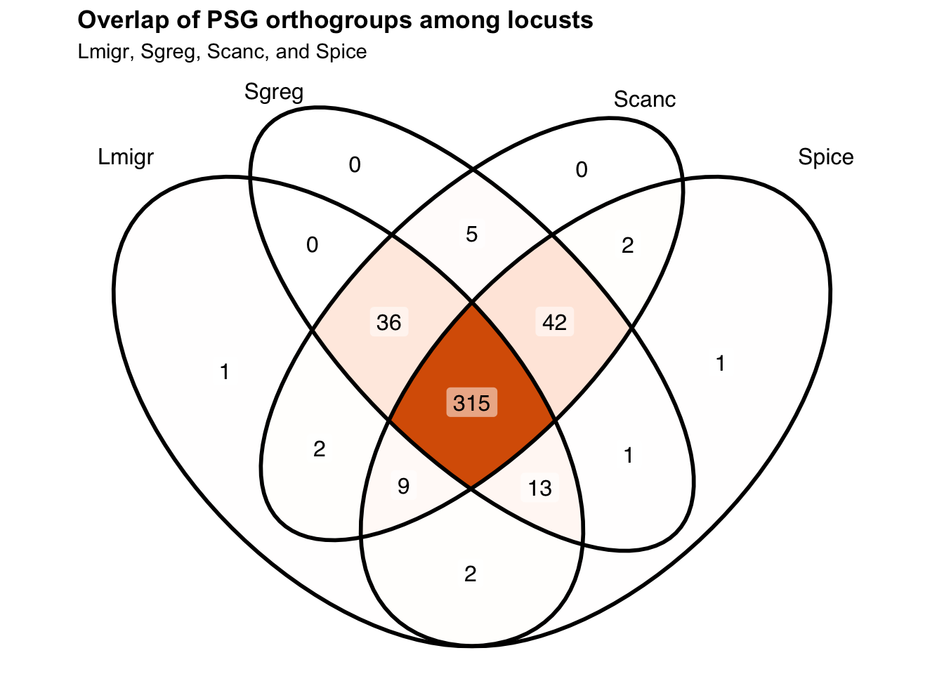
5 7 262locust_psg_shared <- psg_overlap %>%
filter(
Lmigr == 1,
Sgreg == 1,
Scanc == 1,
Spice == 1
)
print(locust_psg_shared)# A tibble: 315 × 8
orthogroup Lmigr Samer Scanc Sgreg Snite Spice Sscub
<chr> <dbl> <dbl> <dbl> <dbl> <dbl> <dbl> <dbl>
1 OG0004349 1 1 1 1 1 1 1
2 OG0004358 1 1 1 1 1 1 1
3 OG0004365 1 1 1 1 1 1 1
4 OG0004368 1 1 1 1 1 1 1
5 OG0004396 1 1 1 1 1 1 1
6 OG0004465 1 1 1 1 1 1 1
7 OG0004478 1 1 1 1 1 1 1
8 OG0004537 1 1 1 1 1 1 1
9 OG0004555 1 1 1 1 1 1 1
10 OG0004570 1 1 1 1 1 1 1
# ℹ 305 more rowsnrow(locust_psg_shared)[1] 315schistocerca_locust_psg_shared <- psg_overlap %>%
filter(
Sgreg == 1,
Scanc == 1,
Spice == 1
)
print(schistocerca_locust_psg_shared)# A tibble: 357 × 8
orthogroup Lmigr Samer Scanc Sgreg Snite Spice Sscub
<chr> <dbl> <dbl> <dbl> <dbl> <dbl> <dbl> <dbl>
1 OG0004349 1 1 1 1 1 1 1
2 OG0004358 1 1 1 1 1 1 1
3 OG0004365 1 1 1 1 1 1 1
4 OG0004368 1 1 1 1 1 1 1
5 OG0004396 1 1 1 1 1 1 1
6 OG0004440 0 1 1 1 1 1 1
7 OG0004465 1 1 1 1 1 1 1
8 OG0004478 1 1 1 1 1 1 1
9 OG0004537 1 1 1 1 1 1 1
10 OG0004555 1 1 1 1 1 1 1
# ℹ 347 more rowsnrow(schistocerca_locust_psg_shared)[1] 357Make a venn diagram with all locusts
library(dplyr)
library(ggVennDiagram)

# Build PSG orthogroup sets for the four locusts
psg_sets_locusts <- dnds_data %>%
  filter(PSG == TRUE, Species %in% c("Lmigr", "Sgreg", "Scanc", "Spice")) %>%
  distinct(Species, orthogroup) %>%
  group_by(Species) %>%
  summarise(orthogroups = list(unique(orthogroup)), .groups = "drop")

venn_list_locusts <- setNames(psg_sets_locusts$orthogroups, psg_sets_locusts$Species)

# Plot
ggVennDiagram(venn_list_locusts, label = "count") +
  scale_fill_gradient(low = "white", high = "#D95F02") +
  labs(
    title = "Overlap of PSG orthogroups among locusts",
    subtitle = "Lmigr, Sgreg, Scanc, and Spice"
  ) +
  theme(
    plot.title = element_text(face = "bold"),
    legend.position = "none"
  )
| Version | Author | Date |
|---|---|---|
| 6e321f0 | Maeva TECHER | 2026-04-06 |
7. aBSREL
Running the analysis
We will perform aBSREL analysis using both unlabeled and labelled phylogeny.
# For Polyneoptera
# For unlabelled phylogeny
sbatch ./scripts/RunaBSREL_May2025.sh \
/scratch/group/songlab/maeva/LocustsGenomeEvolution/Polyneoptera_FINAL/5_OrthoFinder/fasta/Results_May26_iqtree/Resolved_Gene_Trees/ \
/scratch/group/songlab/maeva/LocustsGenomeEvolution/Polyneoptera_FINAL/5_OrthoFinder/fasta/Results_May26_iqtree/Orthogroups/Orthogroups_SingleCopyOrthologues_selanalysiswide.txt

# For labelled phylogeny
sbatch ./scripts/RunaBSREL_labeled_May2025.sh \
/scratch/group/songlab/maeva/LocustsGenomeEvolution/Polyneoptera_FINAL/9_1_LabelledPhylogenies/Locusts \
Locusts \
/scratch/group/songlab/maeva/LocustsGenomeEvolution/Polyneoptera_FINAL/5_OrthoFinder/fasta/Results_May26_iqtree/Orthogroups/Orthogroups_SingleCopyOrthologues_selanalysiswide.txt

# For labelled phylogeny PRUNED
sbatch ./scripts/RunaBSREL_labeled_June2025.sh \
/scratch/group/songlab/maeva/LocustsGenomeEvolution/Polyneoptera_FINAL/9_1_LabelledPhylogenies_Pruned/Locusts \
Locusts \
/scratch/group/songlab/maeva/LocustsGenomeEvolution/Polyneoptera_FINAL/5_OrthoFinder/fasta/Results_May26_iqtree/Orthogroups/Orthogroups_SingleCopyOrthologues_selanalysiswide.txt
Unlabeled
Parsing the json files
For parsing the results, you just do:
srun --ntasks 1 --cpus-per-task 16 --mem 50G --time 05:00:00 --pty bash
ml GCC/13.2.0  OpenMPI/4.1.6 R_tamu/4.4.1
export R_LIBS=$SCRATCH/R_LIBS_USER/

Rscript ./scripts/Parsing_aBSRELresulsr_unlabel_June2025.R
Below is the detail of the parsing aBSREL script
./scripts/Parsing_aBSRELresulsr_unlabel_June2025.R:
# ===========================
# A. LOAD LIBRARIES
# ===========================
library(jsonlite)
library(dplyr)
library(stringr)
library(readr)
library(tibble)

# ===========================
# B. DEFINE PATHS
# ===========================
input_dir <- "/Users/maevatecher/Desktop/Polyneoptera_FINAL/9_2_ABSRELResults_unlabeled/"
output_dir <- "/Users/maevatecher/Desktop/Polyneoptera_FINAL/ParsedABSRELResults_unlabeled/"
orthotable_path <- "/Users/maevatecher/Documents/GitHub/locust-comparative-genomics/data/orthofinder/Polyneoptera/Results_I2_iqtree/Orthogroups/Orthogroups_CladeAssignment_WithCopyStatus_cleaned.csv"

# ===========================
# C. INITIALIZE
# ===========================
files <- list.files(path = input_dir, pattern = "\\.json$", full.names = TRUE)
file_all <- file.path(output_dir, "parsed_absrel_full.csv")
file_sig <- file.path(output_dir, "parsed_absrel_significant_full.csv")

all_results <- data.frame()
sig_results <- data.frame()

# ===========================
# D. PARSE JSON FILES
# ===========================

for (file in files) {
  try({
    json <- fromJSON(file)
    orthogroup <- str_extract(basename(file), "OG[0-9]+")

    # Check required fields exist
    if (!"branch attributes" %in% names(json)) next
    if (!"0" %in% names(json$`branch attributes`)) next

    branches <- json$`branch attributes`$`0`

    # Pull alignment stats once per file
    aln_length <- json$input$`number of sites`
    seq_count  <- json$input$`number of sequences`

    for (branch_name in names(branches)) {
      entry <- branches[[branch_name]]
      rates <- entry$`Rate Distributions`
      n <- if (!is.null(rates)) nrow(as.data.frame(rates)) else 0

      row <- data.frame(
        Orthogroup = orthogroup,
        Branch = branch_name,
        Species = substr(branch_name, 1, 5),
        Baseline_MG94xREV = entry$`Baseline MG94xREV`,
        Baseline_omega = entry$`Baseline MG94xREV omega ratio`,
        Full_adaptive_model = entry$`Full adaptive model`,
        Full_adaptive_model_nonsyn = entry$`Full adaptive model (non-synonymous subs/site)`,
        Full_adaptive_model_syn = entry$`Full adaptive model (synonymous subs/site)`,
        LRT = entry$`LRT`,
        Nucleotide_GTR = entry$`Nucleotide GTR`,
        Rate_classes = entry$`Rate classes`,
        Uncorrected_P = entry$`Uncorrected P-value`,
        Corrected_P = entry$`Corrected P-value`,
        aln_length = aln_length,
        seq_count = seq_count,
        Omega1 = NA, Percent1 = NA,
        Omega2 = NA, Percent2 = NA,
        Omega3 = NA, Percent3 = NA,
        stringsAsFactors = FALSE
      )

      # Add omega/proportion values
      if (!is.null(rates)) {
        df <- as.data.frame(rates)
        for (i in 1:min(n, 3)) {
          row[[paste0("Omega", i)]] <- df[i, 1]
          row[[paste0("Percent", i)]] <- df[i, 2]
        }
      }

      all_results <- bind_rows(all_results, row)

      if (!is.null(row$Corrected_P) && !is.na(row$Corrected_P) && row$Corrected_P <= 0.05) {
        sig_results <- bind_rows(sig_results, row)
      }
    }
  }, silent = TRUE)
}


# ===========================
# E. FLAG SUSPECT BRANCHES
# ===========================
all_results <- all_results %>%
  mutate(
    Baseline_omega = as.numeric(Baseline_omega),
    aln_length = as.numeric(aln_length),
    seq_count = as.numeric(seq_count),
    Suspect_Result = is.na(Baseline_omega) | Baseline_omega > 100 | aln_length < 100 | seq_count < 4
  )

sig_results <- sig_results %>%
  mutate(
    Baseline_omega = as.numeric(Baseline_omega),
    aln_length = as.numeric(aln_length),
    seq_count = as.numeric(seq_count),
    Suspect_Result = is.na(Baseline_omega) | Baseline_omega > 100 | aln_length < 100 | seq_count < 4
  )

# ===========================
# F. WRITE OUTPUT
# ===========================
if (!dir.exists(output_dir)) dir.create(output_dir, recursive = TRUE)
write_csv(all_results, file_all)
write_csv(sig_results, file_sig)
cat("✅ Full parsing complete.\n")

# ===========================
# G. CREATE SUMMARY TABLE
# ===========================
createSummaryTable <- function(results_df) {
  results_df %>%
    mutate(across(starts_with("Omega"), as.numeric),
           Corrected_P = as.numeric(Corrected_P),
           Significant = Corrected_P <= 0.05) %>%
    rowwise() %>%
    mutate(
      Mean_omega = mean(c_across(starts_with("Omega")), na.rm = TRUE),
      Max_omega = max(c_across(starts_with("Omega")), na.rm = TRUE)
    ) %>%
    ungroup() %>%
    group_by(Orthogroup) %>%
    summarise(
      Total_Branches = n(),
      Significant_Branches = sum(Significant),
      Proportion_Significant = Significant_Branches / Total_Branches,
      Suspect_Branches = sum(Suspect_Result),
      Positive_Species = paste0(Species[Significant], collapse = ";"),
      Mean_omega = mean(Mean_omega, na.rm = TRUE),
      Max_omega = max(Max_omega, na.rm = TRUE),
      .groups = "drop"
    )
}

summary_table <- createSummaryTable(all_results)
write_csv(summary_table, file.path(output_dir, "absrel_summary_table.csv"))

# ===========================
# H. ANNOTATE WITH ORTHO INFO
# ===========================
orthologtable <- read_csv(orthotable_path)
absrel_df <- left_join(all_results, orthologtable, by = "Orthogroup") %>%
  mutate(
    Selection = as.numeric(Corrected_P) <= 0.05,
    Category = case_when(
      SelAnalysisStrict == "Included" ~ "1:1 Polyneoptera",
      SelAnalysisLocusts == "Included" ~ "1:1 Caelifera only",
      SelAnalysisMixed == "Included" ~ "1:1 Mixed",
      TRUE ~ "Other"
    )
  ) %>%
  relocate(Orthogroup, Branch, Species, Category, Selection, Corrected_P, starts_with("Omega"))

write_csv(absrel_df, file.path(output_dir, "parsed_absrel_annotated.csv"))

# ===========================
# I. SUMMARY PER SPECIES × CATEGORY
# ===========================
absrel_species_summary <- absrel_df %>%
  group_by(Species, Category) %>%
  summarise(
    Significant_Branches = sum(Selection),
    NonSignificant_Branches = sum(!Selection),
    Suspect_Branches = sum(Suspect_Result),
    Total_Branches = n(),
    .groups = "drop"
  ) %>%
  arrange(Species, Category)

knitr::kable(absrel_species_summary, caption = "Summary of aBSREL results: per species and category")
Plotting the results
library("ggplot2")

# Load annotated aBSREL results
absrel_annotated_df <- read_csv("/Users/maevatecher/Documents/GitHub/locust-comparative-genomics/data/HYPHY_selection/ParsedABSRELResults_unlabeled/parsed_absrel_annotated.csv"
)
output_dir <- "/Users/maevatecher/Documents/GitHub/locust-comparative-genomics/data/HYPHY_selection/ParsedABSRELResults_unlabeled/"

# Ensure Selection is logical and Category is not NA
absrel_clean <- absrel_annotated_df %>%
  filter(!is.na(Category)) %>%
  mutate(
    Selection = as.logical(Selection),
    Category = factor(Category, levels = c("1:1 Polyneoptera", "1:1 Caelifera only", "1:1 Mixed")),
    Species = factor(Species)
  )

# Create summary count table per species × category × selection status
absrel_summary_counts <- absrel_clean %>%
  group_by(Species, Category, Selection) %>%
  summarise(N = n(), .groups = "drop")

# Set factor levels for consistent fill order
absrel_summary_counts$Selection <- factor(
  absrel_summary_counts$Selection,
  levels = c(FALSE, TRUE),
  labels = c("Not Selected", "Selected")
)


# Reorder Species factor
absrel_summary_counts <- absrel_summary_counts %>%
  filter(!Species %in% paste0("n", 1:11)) %>%  # Clean internal nodes in one line
  mutate(Species = factor(Species, levels = c("Pamer", "Csecu", "Brsri",
     "Glong","Gbima", "Asimp", "Sscub","Samer", "Spice", "Scanc", "Snite", "Sgreg",
    "Lmigr"
  )))


# Plot
ggplot(absrel_summary_counts, aes(x = Species, y = N, fill = Selection)) +
  geom_bar(stat = "identity", position = "stack") +
  coord_flip() +  # Flip to horizontal
  facet_wrap(~ Category, ncol = 1, scales = "free_y") +
  scale_fill_manual(values = c("Not Selected" = "#d9d9d9", "Selected" = "#1b9e77")) +
  labs(
    title = "aBSREL Selection Summary per Species and Orthogroup Category",
    x = "Species",
    y = "Number of Branches",
    fill = "Selection Status"
  ) +
  theme_minimal(base_size = 14) +
  theme(
    axis.text.y = element_text(face = "italic"),
    strip.text = element_text(face = "bold")
  )


category_colors <- c(
  "1:1 Polyneoptera" = "gold",
  "1:1 Mixed" = "black",
  "1:1 Caelifera only" = "green3",
  "Not Selected" = "gray90"
)

# Get Not Selected totals
not_selected <- absrel_summary_counts %>%
  filter(Selection == "Not Selected") %>%
  group_by(Species) %>%
  summarise(N = sum(N), Category = "Not Selected", .groups = "drop")

# Bind with selected data
combined_bar_data <- bind_rows(
  absrel_summary_counts %>% filter(Selection == "Selected"),
  not_selected
)

ggplot(combined_bar_data,
       aes(x = Species, y = N, fill = Category)) +
  geom_bar(stat = "identity", position = "stack") +
  coord_flip() +
  scale_fill_manual(values = category_colors) +
  labs(
    title = "Selected Branches per Species",
    subtitle = "Colored by Orthogroup Category",
    x = "Species",
    y = "Number of Selected Branches",
    fill = "Orthogroup Category"
  ) +
  theme_minimal(base_size = 14) +
  theme(
    axis.text.y = element_text(face = "italic"),
    strip.text = element_text(face = "bold")
  )

ggplot(absrel_summary_counts %>% filter(Selection == "Selected"),
       aes(x = Species, y = N, fill = Category)) +
  geom_bar(stat = "identity", position = "stack") +
  coord_flip() +
  scale_fill_manual(values = category_colors) +
  labs(
    title = "Selected Branches per Species",
    subtitle = "Colored by Orthogroup Category",
    x = "Species",
    y = "Number of Selected Branches",
    fill = "Orthogroup Category"
  ) +
  theme_minimal(base_size = 14) +
  theme(
    axis.text.y = element_text(face = "italic"),
    strip.text = element_text(face = "bold")
  )

  ### tree
library(pheatmap)
library(tidyverse)

# Filter significant only
significant_mat <- absrel_annotated_df %>%
  filter(`Corrected_P` <= 0.05) %>%
  mutate(Significant = 1) %>%
  distinct(Orthogroup, Species, Significant) %>%
  pivot_wider(names_from = Orthogroup, values_from = Significant, values_fill = 0) %>%
  column_to_rownames("Species") %>%
  as.matrix()

# Save heatmap
pdf(file.path(output_dir, "heatmap_significant_orthogroups.pdf"), width = 9, height = 6)
pheatmap(significant_mat,
         cluster_rows = TRUE,
         cluster_cols = TRUE,
         color = c("white", "darkred"),
         main = "aBSREL: Positive Selection Heatmap")
dev.off()

library(tidyverse)
library(igraph)

# Define helper function for pairwise combinations
pairwise_combinations <- function(df, col) {
  col <- rlang::ensym(col)
  df %>%
    group_by(!!col) %>%
    filter(n() > 1) %>%
    summarise(pairs = list(t(combn(unique(.[[deparse(col)]]), 2))), .groups = "drop") %>%
    unnest_wider(pairs, names_sep = "_") %>%
    rename(from = pairs_1, to = pairs_2)
}

# Build edge list from significant orthogroups with more than 1 species
#edges <- all_results %>%
#  filter(Corrected_P <= 0.05) %>%
#  distinct(Species, Orthogroup) %>%
#  pairwise_combinations(Orthogroup)

# Create graph object
#g <- graph_from_data_frame(edges, directed = FALSE)

# Optional: plot it
#pdf(file.path(output_dir, "network_positive_selection_species.pdf"), width = 8, height = 8)
#plot(
#  g,
#  vertex.size = 30,
#  vertex.label.cex = 0.9,
#  vertex.label.color = "black",
#  vertex.color = "skyblue",
#  edge.width = ,
#  main = "Network of Species Co-selected in aBSREL Orthogroups"
#)
#dev.off()

acrididae_species <- c(
  "Lmigr", "Sgreg", "Scanc", "Spice",
  "Samer", "Sscub", "Snite"
)

combined_bar_acrididae <- combined_bar_data %>%
  filter(Species %in% acrididae_species)

combined_bar_acrididae_sel <- combined_bar_acrididae %>%
  filter(Category != "Not Selected")

ggplot(combined_bar_acrididae_sel,
       aes(x = Species, y = N, fill = Category)) +

  geom_bar(
    stat = "identity",
    position = "stack",
    width = 0.7,
    color = "black",
    size = 0.2
  ) +

  coord_flip() +

  scale_fill_manual(
    values = category_colors[names(category_colors) != "Not Selected"],
    guide = guide_legend(reverse = TRUE)
  ) +

  labs(
    title = "Selection landscape across Acrididae",
    subtitle = "aBSREL-detected positive selection by orthogroup category",
    x = NULL,
    y = "Number of selected branches",
    fill = "Orthogroup category"
  ) +

  theme_minimal(base_size = 14) +

  theme(
    plot.title = element_text(face = "bold", size = 16, hjust = 0.5),
    plot.subtitle = element_text(size = 12, hjust = 0.5),

    axis.text.y = element_text(face = "italic", size = 12),
    axis.text.x = element_text(size = 11),
    axis.title.x = element_text(face = "bold", size = 12),

    panel.grid.major.y = element_blank(),
    panel.grid.minor = element_blank(),

    legend.position = "right",
    legend.title = element_text(face = "bold"),

    plot.margin = margin(10, 15, 10, 10)
  )

### with not selected


acrididae_species <- c(
  "Lmigr", "Sgreg", "Scanc", "Spice",
  "Samer", "Sscub", "Snite"
)

combined_bar_acrididae <- combined_bar_data %>%
  filter(Species %in% acrididae_species)

ggplot(combined_bar_acrididae,
       aes(x = Species, y = N, fill = Category)) +

  geom_bar(
    stat = "identity",
    position = "stack",
    width = 0.7,
    color = "black",
    size = 0.2
  ) +

  coord_flip() +

  scale_fill_manual(
    values = c(
      category_colors,
      "Not Selected" = "grey80"
    ),
    guide = guide_legend(reverse = TRUE)
  ) +

  labs(
    title = "Selection landscape across Acrididae",
    subtitle = "aBSREL-detected positive selection by orthogroup category",
    x = NULL,
    y = "Number of branches",
    fill = "Orthogroup category"
  ) +

  theme_minimal(base_size = 14) +

  theme(
    plot.title = element_text(face = "bold", size = 16, hjust = 0.5),
    plot.subtitle = element_text(size = 12, hjust = 0.5),

    axis.text.y = element_text(face = "italic", size = 12),
    axis.text.x = element_text(size = 11),
    axis.title.x = element_text(face = "bold", size = 12),

    panel.grid.major.y = element_blank(),
    panel.grid.minor = element_blank(),

    legend.position = "right",
    legend.title = element_text(face = "bold"),

    plot.margin = margin(10, 15, 10, 10)
  )
Warning: The above code chunk cached its results, but
it won’t be re-run if previous chunks it depends on are updated. If you
need to use caching, it is highly recommended to also set
knitr::opts_chunk$set(autodep = TRUE) at the top of the
file (in a chunk that is not cached). Alternatively, you can customize
the option dependson for each individual chunk that is
cached. Using either autodep or dependson will
remove this warning. See the
knitr cache options for more details.
# ===========================
# Load Libraries
# ===========================
library(ape)
Attaching package: 'ape'The following object is masked from 'package:dplyr':
wherelibrary(viridis)Loading required package: viridisLitelibrary(tidyverse)Warning: package 'tibble' was built under R version 4.4.3Warning: package 'purrr' was built under R version 4.4.3── Attaching core tidyverse packages ──────────────────────── tidyverse 2.0.0 ──
✔ forcats 1.0.1 ✔ stringr 1.6.0
✔ lubridate 1.9.4 ✔ tibble 3.3.1
✔ purrr 1.2.1 ── Conflicts ────────────────────────────────────────── tidyverse_conflicts() ──
✖ dplyr::filter() masks stats::filter()
✖ dplyr::lag() masks stats::lag()
✖ ggVennDiagram::unite() masks tidyr::unite()
✖ ape::where() masks dplyr::where()
ℹ Use the conflicted package (<http://conflicted.r-lib.org/>) to force all conflicts to become errors# ===========================
# File Paths
# ===========================
input_results <- "/Users/maevatecher/Documents/GitHub/locust-comparative-genomics/data/HYPHY_selection/ParsedABSRELResults_unlabeled/parsed_absrel_full.csv"
tree_file <- "/Users/maevatecher/Documents/GitHub/locust-comparative-genomics/data/orthofinder/Polyneoptera/Results_I2_iqtree/Species_Tree/SpeciesTree_rooted_node_labels.txt"
output_file <- "/Users/maevatecher/Documents/GitHub/locust-comparative-genomics/data/HYPHY_selection/ParsedABSRELResults_unlabeled/tree_colored_by_omega3_allbranches_FINAL.pdf"
trusted_orthogroups <- readLines("/Users/maevatecher/Documents/GitHub/locust-comparative-genomics/data/orthofinder/Polyneoptera/Results_I2_iqtree/trusted_ogs_v2.txt")
# ===========================
# Load Data
# ===========================
all_results <- read_csv(input_results, show_col_types = FALSE)
filtered_results <- all_results %>%
filter(Suspect_Result == "FALSE") %>%
# filter(Orthogroup %in% trusted_orthogroups) %>%
filter(Orthogroup %in% trusted_orthogroups & !is.na(Baseline_omega))
tree <- read.tree(tree_file)
desired_order <- c(
"Pamer_filteredTranscripts", "Csecu_filteredTranscripts",
"Sgreg_filteredTranscripts", "Snite_filteredTranscripts", "Scanc_filteredTranscripts",
"Spice_filteredTranscripts", "Sscub_filteredTranscripts", "Samer_filteredTranscripts",
"Lmigr_filteredTranscripts", "Asimp_filteredTranscripts", "Glong_filteredTranscripts",
"Gbima_filteredTranscripts", "Brsri_filteredTranscripts"
)
desired_order <- c(
"Pamer", "Csecu",
"Sgreg", "Snite", "Scanc",
"Spice", "Sscub", "Samer",
"Lmigr", "Asimp", "Glong",
"Gbima", "Brsri"
)
# Ensure all desired tips are in the tree
stopifnot(all(desired_order %in% tree$tip.label))
# Ladderize and reorder the tip labels by desired order
tree <- ladderize(tree, right = FALSE)
# Reorder tree$tip.label visually via `plot.phylo()` call
tip_order <- match(tree$tip.label, desired_order)
# ===========================
# Harmonize Labels
# ===========================
# Create node label lookup: node index → cleaned label
node_labels <- c(tree$tip.label, tree$node.label)
names(node_labels) <- 1:(length(tree$tip.label) + tree$Nnode)
# Remove "_filteredTranscripts..." and lowercase
node_to_label <- tolower(gsub("_filteredTranscripts.*", "", node_labels))
names(node_to_label) <- names(node_labels)
# Clean Branch names from all_results
omega_df <- filtered_results %>%
filter(!is.na(Omega1)) %>%
mutate(label = tolower(gsub("_filteredTranscripts.*", "", Branch))) %>%
group_by(label) %>%
summarize(mean_omega = mean(as.numeric(Omega3), na.rm = TRUE)) %>%
ungroup()
omega_df <- omega_df %>% filter(label != "n2") %>%
filter(label != "n3") %>%
filter(label != "n4") %>%
filter(label != "n5") %>%
filter(label != "n6") %>%
filter(label != "n7") %>%
filter(label != "n8") %>%
filter(label != "n9") %>%
filter(label != "n10") %>%
filter(label != "n11") %>%
filter(label != "asimp") %>%
filter(label != "brsri") %>%
filter(label != "csecu") %>%
filter(label != "gbima") %>%
filter(label != "glong") %>%
filter(label != "pamer")
# ===========================
# Map omega3 to Tree Branches
# ===========================
omega_vals <- rep(NA, nrow(tree$edge))
for (i in seq_len(nrow(tree$edge))) {
child_node <- tree$edge[i, 2]
label <- node_to_label[as.character(child_node)]
if (!is.na(label) && label %in% omega_df$label) {
omega_vals[i] <- omega_df$mean_omega[omega_df$label == label]
}
}
# ===========================
# Generate Colors
# ===========================
color_scale <- viridis(100)
if (all(is.na(omega_vals))) {
warning("No omega values matched any tree node labels.")
edge_colors <- rep("grey", length(omega_vals))
} else {
omega_vals <- as.numeric(omega_vals)
cut_omega <- cut(omega_vals, breaks = 100)
edge_colors <- color_scale[as.numeric(cut_omega)]
edge_colors[is.na(edge_colors)] <- "grey"
}
# ===========================
# Plot Tree with Edge Colors
# ===========================
pdf(output_file, width = 9, height = 7)
par(mar = c(5, 4, 4, 6)) # leave space for legend
plot(tree,
edge.color = edge_colors,
edge.width = 4,
cex = 1,
main = "Mean Omega3 per Branch (Tips + Internal)",
show.tip.label = TRUE,
use.edge.length = FALSE,
tip.order = tip_order)Warning in plot.window(...): "tip.order" is not a graphical parameterWarning in plot.xy(xy, type, ...): "tip.order" is not a graphical parameterWarning in title(...): "tip.order" is not a graphical parameter# Continuous legend (manual)
zlim_vals <- range(omega_vals, na.rm = TRUE)
legend_vals <- pretty(zlim_vals, n = 5)
legend_colors <- color_scale[as.numeric(cut(legend_vals, breaks = 100))]
legend("topright",
legend = round(legend_vals, 2),
fill = legend_colors,
border = NA,
title = "omega")
dev.off()quartz_off_screen
2 message("✅ Tree plot saved to: ", output_file)✅ Tree plot saved to: /Users/maevatecher/Documents/GitHub/locust-comparative-genomics/data/HYPHY_selection/ParsedABSRELResults_unlabeled/tree_colored_by_omega3_allbranches_FINAL.pdfAnnotating OGs under selection
Here we are working with Orthogroups number under selection per branch, and we want to have a functional enrichment of the genes associated per species to allow comparison. First we need to extract the positively selected genes/orthogroups for each species:
library(dplyr)
library(readr)

# Load aBSREL results
absrel_df <- read_csv("/Users/maevatecher/Documents/GitHub/locust-comparative-genomics/data/HYPHY_selection/ParsedABSRELResults_unlabeled/parsed_absrel_annotated.csv")
Rows: 101716 Columns: 44
── Column specification ────────────────────────────────────────────────────────
Delimiter: ","
chr (10): Orthogroup, Branch, Species, Category, Assigned_Clade, Orthogroup_...
dbl (32): Corrected_P, Omega1, Omega2, Omega3, Baseline_MG94xREV, Baseline_o...
lgl (2): Selection, Suspect_Result
ℹ Use `spec()` to retrieve the full column specification for this data.
ℹ Specify the column types or set `show_col_types = FALSE` to quiet this message.# Filter PSGs: significant, non-suspect
psg_ogs <- absrel_df %>%
filter(Selection == TRUE, Suspect_Result == FALSE) %>%
dplyr::select(Species, Orthogroup)
ortho_dir <- "/Users/maevatecher/Documents/GitHub/locust-comparative-genomics/data/orthofinder/Polyneoptera"
input_file <- file.path(ortho_dir, "Results_I2_iqtree/Orthogroups_genesproteinbiotype_13species_annotated_May2025.csv")
ortho_map <- read.csv(input_file, header = TRUE, stringsAsFactors = FALSE)
head(ortho_map) Orthogroup SpeciesID protein_id GeneID
1 OG0000000 Asimp_filteredTranscripts XP_067003642.2 LOC136874043
2 OG0000000 Asimp_filteredTranscripts XP_067004661.1 LOC136874869
3 OG0000000 Asimp_filteredTranscripts XP_067015293.1 LOC136886419
4 OG0000000 Asimp_filteredTranscripts XP_067015651.2 LOC136886746
5 OG0000000 Asimp_filteredTranscripts XP_068085770.1 LOC137496902
6 OG0000000 Asimp_filteredTranscripts XP_068087037.1 LOC137503369
Description Species GeneType
1 farnesol dehydrogenase isoform X1 Asimp protein-coding
2 dehydrogenase/reductase SDR family member 11 Asimp protein-coding
3 farnesol dehydrogenase Asimp protein-coding
4 farnesol dehydrogenase Asimp protein-coding
5 farnesol dehydrogenase-like Asimp protein-coding
6 farnesol dehydrogenase-like Asimp protein-coding
Accession Begin End Orthogroup_Type
1 NC_090269.1 316521124 316596183 MultiCopy
2 NC_090269.1 316408775 316497937 MultiCopy
3 NC_090279.1 165240845 165292312 MultiCopy
4 NC_090279.1 164532314 164617967 MultiCopy
5 NC_090275.1 60074551 60101839 MultiCopy
6 NC_090279.1 164618824 164719067 MultiCopy# Join PSG orthogroups with gene IDs, species-aware
psg_genes <- psg_ogs %>%
inner_join(ortho_map, by = c("Orthogroup","Species")) %>%
dplyr::select(Species, Orthogroup, GeneID)Then we use the same function we used for DEGs GO terms and KEGG enrichment:
# === Paths and Constants ===
workDir     <- "/Users/maevatecher/Documents/GitHub/locust-comparative-genomics/data"
GODir       <- file.path(workDir, "list", "GO_Annotations")
RefDir      <- file.path(workDir, "RefSeq")
enrichDir   <- file.path(workDir, "HYPHY_selection/functional_pathways/aBSREL")
selListDir <- file.path(workDir, "HYPHY_selection/ParsedABSRELResults_unlabeled")

species_list <- c("gregaria", "cancellata", "piceifrons", "americana", "cubense", "nitens")

# === Load Required Libraries ===
library(data.table)
Warning: package 'data.table' was built under R version 4.4.3
Attaching package: 'data.table'The following objects are masked from 'package:lubridate':
hour, isoweek, isoyear, mday, minute, month, quarter, second, wday,
week, yday, yearThe following object is masked from 'package:purrr':
transposeThe following objects are masked from 'package:dplyr':
between, first, lastlibrary(dplyr)
library(readr)
library(clusterProfiler)clusterProfiler v4.14.6 Learn more at https://yulab-smu.top/contribution-knowledge-mining/
Please cite:
T Wu, E Hu, S Xu, M Chen, P Guo, Z Dai, T Feng, L Zhou, W Tang, L Zhan,
X Fu, S Liu, X Bo, and G Yu. clusterProfiler 4.0: A universal
enrichment tool for interpreting omics data. The Innovation. 2021,
2(3):100141
Attaching package: 'clusterProfiler'The following object is masked from 'package:purrr':
simplifyThe following object is masked from 'package:stats':
filterlibrary(GO.db)Loading required package: AnnotationDbiLoading required package: stats4Loading required package: BiocGenerics
Attaching package: 'BiocGenerics'The following objects are masked from 'package:lubridate':
intersect, setdiff, unionThe following objects are masked from 'package:dplyr':
combine, intersect, setdiff, unionThe following objects are masked from 'package:stats':
IQR, mad, sd, var, xtabsThe following objects are masked from 'package:base':
anyDuplicated, aperm, append, as.data.frame, basename, cbind,
colnames, dirname, do.call, duplicated, eval, evalq, Filter, Find,
get, grep, grepl, intersect, is.unsorted, lapply, Map, mapply,
match, mget, order, paste, pmax, pmax.int, pmin, pmin.int,
Position, rank, rbind, Reduce, rownames, sapply, saveRDS, setdiff,
table, tapply, union, unique, unsplit, which.max, which.minLoading required package: BiobaseWelcome to Bioconductor
Vignettes contain introductory material; view with
'browseVignettes()'. To cite Bioconductor, see
'citation("Biobase")', and for packages 'citation("pkgname")'.Loading required package: IRangesLoading required package: S4Vectors
Attaching package: 'S4Vectors'The following object is masked from 'package:clusterProfiler':
renameThe following objects are masked from 'package:data.table':
first, secondThe following objects are masked from 'package:lubridate':
second, second<-The following object is masked from 'package:tidyr':
expandThe following objects are masked from 'package:dplyr':
first, renameThe following object is masked from 'package:utils':
findMatchesThe following objects are masked from 'package:base':
expand.grid, I, unname
Attaching package: 'IRanges'The following object is masked from 'package:clusterProfiler':
sliceThe following object is masked from 'package:data.table':
shiftThe following object is masked from 'package:lubridate':
%within%The following object is masked from 'package:purrr':
reduceThe following objects are masked from 'package:dplyr':
collapse, desc, slice
Attaching package: 'AnnotationDbi'The following object is masked from 'package:clusterProfiler':
selectThe following object is masked from 'package:dplyr':
selectlibrary(rtracklayer)Loading required package: GenomicRangesLoading required package: GenomeInfoDblibrary(DesertLocustR) # Local installationLoading required package: AnnotationHubLoading required package: BiocFileCacheLoading required package: dbplyr
Attaching package: 'dbplyr'The following objects are masked from 'package:dplyr':
ident, sql
Attaching package: 'AnnotationHub'The following object is masked from 'package:rtracklayer':
hubUrlThe following object is masked from 'package:Biobase':
cacheLoading required package: BiostringsLoading required package: XVector
Attaching package: 'XVector'The following object is masked from 'package:purrr':
compact
Attaching package: 'Biostrings'The following object is masked from 'package:ape':
complementThe following object is masked from 'package:base':
strsplitLoading required package: remotesgff_map <- c(
gregaria = "GCF_023897955.1_iqSchGreg1.2_genomic.gff",
cancellata = "GCF_023864275.1_iqSchCanc2.1_genomic.gff",
piceifrons = "GCF_021461385.2_iqSchPice1.1_genomic.gff",
americana = "GCF_021461395.2_iqSchAmer2.1_genomic.gff",
cubense = "GCF_023864345.2_iqSchSeri2.2_genomic.gff",
nitens = "GCF_023898315.1_iqSchNite1.1_genomic.gff"
)
annot_map <- c(
gregaria = "EggNog_Arthropoda_one2one.emapper.annotations",
cancellata = "GCF_023864275.1_iqSchCanc2.1_Arthopoda_one2one.emapper.annotations",
piceifrons = "GCF_021461385.2_iqSchPice1.1_Arthopoda_one2one.emapper.annotations",
americana = "GCF_021461395.2_iqSchAmer2.1_Arthopoda_one2one.emapper.annotations",
cubense = "GCF_023864345.2_iqSchSeri2.2_Arthopoda_one2one.emapper.annotations",
nitens = "GCF_023898315.1_iqSchNite1.1_Arthopoda_one2one.emapper.annotations"
)
# GO enrichment
enrich_GO <- function(dge_genes.df, term2gene, term2name, pval, qval){
genes <- rownames(dge_genes.df)
enricher(genes, TERM2GENE = term2gene, TERM2NAME = term2name, pvalueCutoff = pval,
pAdjustMethod = "BH", qvalueCutoff = qval)
}
# KEGG preparation
assign_kegg_ids <- function(sig_genes.df){
if (is.vector(sig_genes.df)) {
sig_genes.df <- data.frame(X.query = sig_genes.df, stringsAsFactors = FALSE)
} else {
sig_genes.df$X.query <- rownames(sig_genes.df)
}
dge_with_kegg_ids <- left_join(sig_genes.df, kegg_final, by = "X.query")
dge_with_kegg_ids$KEGG_ko[grepl("^K", dge_with_kegg_ids$KEGG_ko)]
}
# KEGG enrichment
enrich_KEGG <- function(dge_genes.df, pval_cutoff = 0.05, qval_cutoff = 0.05) {
gene_with_kegg_ids <- assign_kegg_ids(dge_genes.df)
enrichKEGG(
gene = gene_with_kegg_ids,
organism = "ko",
pvalueCutoff = pval_cutoff,
qvalueCutoff = qval_cutoff,
pAdjustMethod = "BH"
)
}
run_GO_enrichment_selected <- function(
gene_list,
go_table,
term2name,
species,
suffix,
ontology,
output_dir,
show_n = 30,
top_n = 30
) {
if (length(gene_list) == 0) return(NULL)
if (!dir.exists(output_dir)) {
dir.create(output_dir, recursive = TRUE)
}
# Make sure column names are correct for clusterProfiler::enricher()
go_table_fixed <- go_table[, 1:2]
colnames(go_table_fixed) <- c("go_id", "gene_id")
term2name_fixed <- term2name[, 1:2]
colnames(term2name_fixed) <- c("go_id", "name")
# Run enrichment
go_result <- enricher(
gene = gene_list,
TERM2GENE = go_table_fixed,
TERM2NAME = term2name_fixed,
pvalueCutoff = 0.05,
qvalueCutoff = 0.05
)
if (!is.null(go_result) &&
inherits(go_result, "enrichResult") &&
nrow(go_result@result) > 0 &&
sum(!is.na(go_result@result$Description)) > 0) {
# Save dotplot
try({
pdf(file = file.path(output_dir, paste0("GO_", ontology, "_dotplot_", species, "_", suffix, ".pdf")),
width = 8, height = 6)
print(dotplot(go_result, showCategory = min(show_n, nrow(go_result@result))) +
ggtitle(paste(ontology, suffix)))
dev.off()
}, silent = TRUE)
# Export top terms with log10(p)
species_enrich_ready <- go_result@result[, c("ID", "p.adjust")]
species_enrich_ready$logp <- -log10(species_enrich_ready$p.adjust)
species_enrich_ready <- species_enrich_ready[order(-species_enrich_ready$logp), ]
species_enrich_ready <- head(species_enrich_ready, n = top_n)[, c("ID", "logp")]
write.table(species_enrich_ready,
file = file.path(output_dir, paste0("enrich_", ontology, "_GOs_", species, "_", suffix, ".txt")),
sep = "\t", quote = FALSE, row.names = FALSE, col.names = FALSE)
# Also export the full table if needed
write.csv(go_result@result,
file = file.path(output_dir, paste0("GO_enrichment_full_", ontology, "_", species, "_", suffix, ".csv")),
row.names = FALSE)
} else {
message(paste0("⚠️ No GO enrichment result to plot/export for ", species, " - ", suffix))
}
}
run_KEGG_enrichment_selected <- function(gene_list, species, suffix, output_dir,
show_n = 40, top_n = 40) {
if (length(gene_list) == 0) return(NULL)
kegg_result <- enrich_KEGG(gene_list, pval_cutoff = 0.05, qval_cutoff = 0.05)
if (!is.null(kegg_result) && inherits(kegg_result, "enrichResult") &&
nrow(kegg_result@result) > 0) {
try({
pdf(file = file.path(output_dir, paste0("KEGG_dotplot_", species, "_", suffix, ".pdf")),
width = 8, height = 6)
print(dotplot(kegg_result, showCategory = min(show_n, nrow(kegg_result@result))) +
ggtitle(paste("KEGG", suffix)))
dev.off()
}, silent = TRUE)
# Full result
write.csv(kegg_result@result,
file = file.path(output_dir, paste0("KEGG_enrichment_", species, "_", suffix, ".csv")),
row.names = FALSE)
# Top KEGG terms
species_enrich_kegg <- kegg_result@result[, c("ID", "p.adjust")]
species_enrich_kegg$logp <- -log10(species_enrich_kegg$p.adjust)
species_enrich_kegg <- species_enrich_kegg[order(-species_enrich_kegg$logp), ][1:min(nrow(species_enrich_kegg), top_n), ]
species_enrich_kegg <- species_enrich_kegg[, c("ID", "logp")]
write.table(species_enrich_kegg,
file = file.path(output_dir, paste0("enrich_KEGG_", species, "_", suffix, ".txt")),
sep = "\t", quote = FALSE, row.names = FALSE, col.names = FALSE)
} else {
message(paste("⚠️ No KEGG enrichment result to plot/export for", species, "-", suffix))
}
}
GO_terms_list <- list()
ontologies_list <- list()
term2name_list <- list()
kegg_final_list <- list()
# Mapping external species names to internal codes in ortho_map
species_translate <- c(
gregaria = "Sgreg",
cancellata = "Scanc",
piceifrons = "Spice",
americana = "Samer", # double-check this is correct
cubense = "Sscub",
nitens = "Snite"
)
for (sp in species_list) {
message("Preparing annotations for ", sp)
sp_code <- species_translate[sp]
eggnog_path <- file.path(GODir, annot_map[[sp]])
gff_path <- file.path(RefDir, gff_map[[sp]])
output_dir <- file.path(enrichDir, sp)
dir.create(output_dir, recursive = TRUE, showWarnings = FALSE)
eggnog_annots <- read.delim(eggnog_path, sep = "\t", skip = 4)
eggnog_annots <- eggnog_annots[1:(nrow(eggnog_annots) - 3), ]
gff.df <- as.data.frame(import(gff_path))
protein_2_gene <- unique(gff.df[c("Name", "gene")])
protein_2_gene_df <- subset(protein_2_gene, grepl("^XP", protein_2_gene$Name))
eggnog_annots$Name <- eggnog_annots$X.query
eggnog_annots <- left_join(eggnog_annots, protein_2_gene_df, by = "Name")
eggnog_annots$X.query <- eggnog_annots$gene
# GO
GO_terms <- data.table(eggnog_annots[, c("X.query", "GOs")])
GO_terms <- GO_terms[, .(GOs = unlist(strsplit(GOs, ","))), by = X.query]
term2name <- GO_terms[, .(GOs, X.query)]
term2name$Names <- mapIds(GO.db, keys = term2name$GOs, column = "TERM", keytype = "GOID")
term2name$Ontology <- mapIds(GO.db, keys = term2name$GOs, column = "ONTOLOGY", keytype = "GOID")
term2name <- as.data.frame(term2name)
go_bp <- term2name[term2name$Ontology == "BP", c("GOs", "X.query")]
go_mf <- term2name[term2name$Ontology == "MF", c("GOs", "X.query")]
go_cc <- term2name[term2name$Ontology == "CC", c("GOs", "X.query")]
term2name_filtered <- term2name[!is.na(term2name$Names), c("GOs", "Names")]
ontologies <- list(BP = go_bp, MF = go_mf, CC = go_cc)
# KEGG
KO_terms <- data.table(eggnog_annots[, c("X.query", "KEGG_ko")])
KO_terms$KEGG_ko <- gsub("ko:", "", as.character(KO_terms$KEGG_ko))
KO_terms <- KO_terms[, .(KEGG_ko = unlist(strsplit(KEGG_ko, ","))), by = X.query]
kegg_final <- KO_terms[, .(KEGG_ko, X.query)]
# Store per species
GO_terms_list[[sp]] <- GO_terms
ontologies_list[[sp]] <- ontologies
term2name_list[[sp]] <- term2name_filtered
kegg_final_list[[sp]] <- kegg_final
}Preparing annotations for gregaria'select()' returned 1:1 mapping between keys and columns
'select()' returned 1:1 mapping between keys and columnsPreparing annotations for cancellata'select()' returned 1:1 mapping between keys and columns
'select()' returned 1:1 mapping between keys and columnsPreparing annotations for piceifrons'select()' returned 1:1 mapping between keys and columns
'select()' returned 1:1 mapping between keys and columnsPreparing annotations for americana'select()' returned 1:1 mapping between keys and columns
'select()' returned 1:1 mapping between keys and columnsPreparing annotations for cubense'select()' returned 1:1 mapping between keys and columns
'select()' returned 1:1 mapping between keys and columnsPreparing annotations for nitens'select()' returned 1:1 mapping between keys and columns
'select()' returned 1:1 mapping between keys and columnsWe run the loop using the list of selected genes extracted in step 1:
# ===== Set up parameters =====
species_list <- c("gregaria", "cancellata", "piceifrons", "americana", "cubense", "nitens")
suffix <- "aBSREL"
# Mapping external species names to internal codes in ortho_map
species_translate <- c(
gregaria = "Sgreg",
cancellata = "Scanc",
piceifrons = "Spice",
americana = "Samer", # double-check this is correct
cubense = "Sscub",
nitens = "Snite"
)
# ===== Loop through each species =====
go_results_all <- list()
kegg_results_all <- list()
# initialize diagnostic log
diagnostic_log <- data.frame(
Species = character(),
PSG_genes = integer(),
GO_overlap = integer(),
KEGG_overlap = integer(),
stringsAsFactors = FALSE
)
for (sp in species_list) {
message("Processing ", sp)
sp_code <- species_translate[sp]
output_dir <- file.path(enrichDir, sp)
dir.create(output_dir, recursive = TRUE, showWarnings = FALSE)
# 1. Extract PSG GeneIDs for this species
species_genes <- psg_genes %>%
filter(Species == sp_code) %>%
pull(GeneID) %>%
unique()
n_psg <- length(species_genes)
message("→ ", n_psg, " PSG genes in ", sp)
# 2. Check overlaps with GO and KEGG annotations
go_annot <- GO_terms_list[[sp]]$X.query
kegg_annot <- kegg_final_list[[sp]]$X.query # ✅ use the correct list
go_overlap <- sum(species_genes %in% go_annot)
kegg_overlap <- sum(species_genes %in% kegg_annot)
message("→ Overlap counts: GO = ", go_overlap, ", KEGG = ", kegg_overlap)
if (kegg_overlap == 0) {
message(" ⚠️ No KEGG matches for ", sp,
". Example missing IDs: ",
paste(head(setdiff(species_genes, kegg_annot), 5), collapse = ", "))
}
# Add to diagnostic log
diagnostic_log <- rbind(diagnostic_log, data.frame(
Species = sp,
PSG_genes = n_psg,
GO_overlap = go_overlap,
KEGG_overlap = kegg_overlap
))
# 3. Run GO enrichment (by ontology)
selected_genes_go <- species_genes[species_genes %in% go_annot]
go_by_onto <- list()
for (onto in names(ontologies_list[[sp]])) {
go_by_onto[[onto]] <- run_GO_enrichment_selected(
gene_list = selected_genes_go,
go_table = ontologies_list[[sp]][[onto]],
term2name = term2name_list[[sp]],
species = sp,
suffix = suffix,
ontology = onto,
output_dir = output_dir
)
}
go_results_all[[sp]] <- go_by_onto
# 4. Run KEGG enrichment
selected_genes_kegg <- species_genes[species_genes %in% kegg_annot]
kegg_final <<- kegg_final_list[[sp]] # required by assign_kegg_ids()
kegg_results_all[[sp]] <- run_KEGG_enrichment_selected(
gene_list = selected_genes_kegg,
species = sp,
suffix = suffix,
output_dir = output_dir
)
}Processing gregaria→ 229 PSG genes in gregaria→ Overlap counts: GO = 197, KEGG = 197Reading KEGG annotation online: "https://rest.kegg.jp/link/ko/pathway"...Reading KEGG annotation online: "https://rest.kegg.jp/list/pathway/ko"...Processing cancellata→ 280 PSG genes in cancellata→ Overlap counts: GO = 252, KEGG = 252Processing piceifrons→ 347 PSG genes in piceifrons→ Overlap counts: GO = 321, KEGG = 321Processing americana→ 222 PSG genes in americana→ Overlap counts: GO = 197, KEGG = 197Processing cubense→ 206 PSG genes in cubense→ Overlap counts: GO = 188, KEGG = 188Processing nitens→ 285 PSG genes in nitens→ Overlap counts: GO = 256, KEGG = 256# save diagnostic log
write.csv(diagnostic_log, file.path(enrichDir, "diagnostic_overlap_log.csv"), row.names = FALSE)
print(diagnostic_log) Species PSG_genes GO_overlap KEGG_overlap
1 gregaria 229 197 197
2 cancellata 280 252 252
3 piceifrons 347 321 321
4 americana 222 197 197
5 cubense 206 188 188
6 nitens 285 256 256Overlap aBSREL locusts
library(dplyr)
library(readr)
library(ggVennDiagram)
library(knitr)
library(kableExtra)
# Load annotated aBSREL results
absrel_df <- read_csv(
"/Users/maevatecher/Documents/GitHub/locust-comparative-genomics/data/HYPHY_selection/ParsedABSRELResults_unlabeled/parsed_absrel_annotated.csv"
)
# Optional: load trusted orthogroups if you want to restrict to your curated set
trusted_orthogroups <- readLines(
"/Users/maevatecher/Documents/GitHub/locust-comparative-genomics/data/orthofinder/Polyneoptera/Results_I2_iqtree/trusted_ogs_v2.txt"
)
# Define the four locusts
locust_species <- c("Lmigr", "Sgreg", "Scanc", "Spice")
# Keep only significant, non-suspect, locust terminal branches
absrel_locust_selected <- absrel_df %>%
filter(
Species %in% locust_species,
Selection == TRUE,
Suspect_Result == FALSE
# Uncomment if you want to restrict to trusted OGs
# , Orthogroup %in% trusted_orthogroups
) %>%
distinct(Species, Orthogroup)
# Build list for Venn diagram
venn_list_absrel <- absrel_locust_selected %>%
group_by(Species) %>%
summarise(orthogroups = list(sort(unique(Orthogroup))), .groups = "drop")
venn_list_absrel <- setNames(venn_list_absrel$orthogroups, venn_list_absrel$Species)
# Optional: prettier labels for the plot
names(venn_list_absrel) <- c(
"L. migratoria",
"S. gregaria",
"S. cancellata",
"S. piceifrons"
)
# Plot Venn
p_absrel_venn <- ggVennDiagram(
venn_list_absrel,
label = "count",
label_alpha = 0,
label_size = 6,
edge_size = 0.5
)
# Make labels bold and lines thinner
p_absrel_venn$layers[[3]]$aes_params$fontface <- "bold"
p_absrel_venn$layers[[1]]$aes_params$size <- 0.4
p_absrel_venn +
scale_fill_gradient(low = "white", high = "antiquewhite") +
labs(
title = "Orthogroups under aBSREL selection shared among locusts",
subtitle = "Significant, non-suspect terminal branches"
) +
theme_void(base_size = 15) +
theme(
plot.title = element_text(face = "bold", size = 16, hjust = 0.5),
plot.subtitle = element_text(size = 12, hjust = 0.5),
legend.position = "none"
)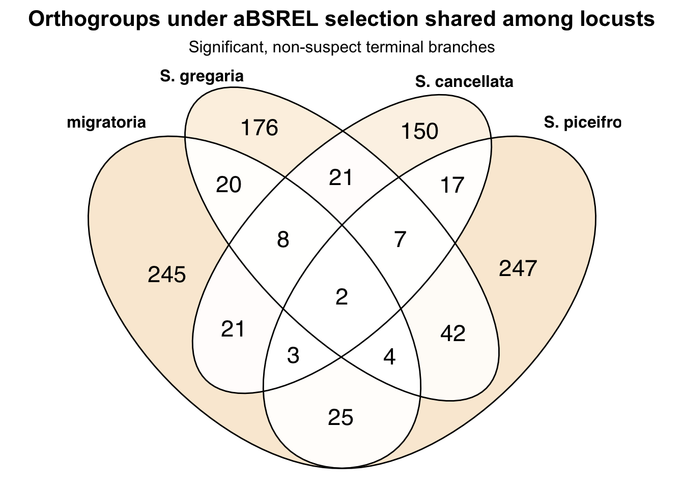
| Version | Author | Date |
|---|---|---|
| 6e321f0 | Maeva TECHER | 2026-04-06 |
Extract orthogroups shared by all four locusts
# Rebuild the set list with short names for downstream extraction
venn_list_absrel_short <- absrel_locust_selected %>%
group_by(Species) %>%
summarise(orthogroups = list(sort(unique(Orthogroup))), .groups = "drop")
venn_list_absrel_short <- setNames(
venn_list_absrel_short$orthogroups,
venn_list_absrel_short$Species
)
# Orthogroups shared by all four locusts
shared_absrel_all_locusts <- Reduce(intersect, venn_list_absrel_short)
length(shared_absrel_all_locusts)[1] 2shared_absrel_all_locusts[1] "OG0011987" "OG0012186"Summary of overlap counts
absrel_overlap_summary <- absrel_locust_selected %>%
distinct(Species, Orthogroup) %>%
count(Orthogroup, name = "n_species") %>%
count(n_species, name = "n_orthogroups") %>%
arrange(n_species)
absrel_overlap_summary %>%
kable(
caption = "Number of orthogroups under aBSREL selection shared across locust species"
) %>%
kable_styling(
bootstrap_options = c("striped", "hover", "condensed"),
full_width = FALSE
)| n_species | n_orthogroups |
|---|---|
| 1 | 818 |
| 2 | 146 |
| 3 | 22 |
| 4 | 2 |
8. BUSTED
We will perform BUSTED analysis using both unlabeled and labelled phylogeny.
The unlabeled gene tree phylogeny will allow for an exploratory analysis, testing all Polyneoptera for positive selection. While this approach provides a broad overview, it comes at the cost of reduced statistical power due to multiple testing.
In contrast, the labelled gene tree phylogeny will focus specifically on migratory locust species compared to all other species or to non-migratory grasshoppers, enabling us to associate traits with selective pressures.
Note: The new version of OrthoFinder
makes a list of SingleCopy Orthologues by adding a N0:H
before the orthogroup name. N0.HOG0000086 N0.HOG0000090 N0.HOG0000212
N0.HOG0000220 N0.HOG0000478 N0.HOG0000479 N0.HOG0000503
N0.HOG0000505
So we need to clean that up before running our files using the command
sed 's/^N0\.HOG/OG/' Orthogroups_SingleCopyOrthologues.txt > Orthogroups_SingleCopyOrthologues_renamed.txtRunning the analysis
We will perform BUSTED analysis using both unlabeled and labelled gene tree phylogeny. The unlabeled phylogeny will allow for a gene-wide exploratory analysis treating the entire tree of Polyneoptera as foreground.
# For Polyneoptera
# For unlabelled phylogeny
sbatch scripts/RunBUSTED_May2025.sh \
/scratch/group/songlab/maeva/LocustsGenomeEvolution/Polyneoptera_FINAL/5_OrthoFinder/fasta/Results_May26_iqtree/Resolved_Gene_Trees/ \
/scratch/group/songlab/maeva/LocustsGenomeEvolution/Polyneoptera_FINAL/5_OrthoFinder/fasta/Results_May26_iqtree/Orthogroups/Orthogroups_SingleCopyOrthologues_selanalysiswide.txt
# For labelled phylogeny
sbatch ./scripts/RunBUSTED_labeled_May2025.sh \
/scratch/group/songlab/maeva/LocustsGenomeEvolution/Polyneoptera_FINAL/9_1_LabelledPhylogenies/Locusts \
Locusts \
/scratch/group/songlab/maeva/LocustsGenomeEvolution/Polyneoptera_FINAL/5_OrthoFinder/fasta/Results_May26_iqtree/Orthogroups/Orthogroups_SingleCopyOrthologues_selanalysiswide.txt
# For labelled phylogeny PRUNED
sbatch ./scripts/RunBUSTED_labeled_June2025.sh \
/scratch/group/songlab/maeva/LocustsGenomeEvolution/Polyneoptera_FINAL/9_1_LabelledPhylogenies_Pruned/Locusts \
Locusts \
/scratch/group/songlab/maeva/LocustsGenomeEvolution/Polyneoptera_FINAL/5_OrthoFinder/fasta/Results_May26_iqtree/Orthogroups/Orthogroups_SingleCopyOrthologues_selanalysiswide.txt If we want to run R interactively on the cluster:
srun --ntasks 1 --cpus-per-task 16 --mem 50G --time 05:00:00 --pty bash
ml GCC/13.2.0 OpenMPI/4.1.6 R_tamu/4.4.1
ml WebProxy
export R_LIBS=$SCRATCH/R_LIBS_USER/
Rscript ./scripts/Parsing_BUSTEDresulsr_unlabel_June2025.RUnlabelled
Parsing the json files
To parse all the details from the BUSTED by testing all branches to
see if we have selection pressures
./scripts/Parsing_BUSTEDresulsr_unlabel_June2025.R:
library(jsonlite)
library(tidyverse)
library(hexbin)
# ============ SETTINGS ============
input_dir <- "/Users/maevatecher/Desktop/Polyneoptera_FINAL/8_3_BustedResults"
single_copy_file <- "/Users/maevatecher/Documents/GitHub/locust-comparative-genomics/data/orthofinder/Polyneoptera/Results_I2_iqtree/Orthogroups/Orthogroups_SingleCopyOrthologues_selanalysiswide.txt"
output_dir <- "/Users/maevatecher/Desktop/Polyneoptera_FINAL/ParsedBUSTEDResults_unlabeled"
dir.create(output_dir, showWarnings = FALSE, recursive = TRUE)
# ============ JSON PARSER ============
parse_busted <- function(file) {
tryCatch({
busted <- jsonlite::fromJSON(file)
og <- stringr::str_extract(basename(file), "^OG[0-9]+")
busted_input_file <- busted[["input"]][["file name"]]
busted_pval <- as.numeric(busted[["test results"]][["p-value"]])
# Corrected metadata fields
aln_length <- busted[["input"]][["number of sites"]]
seq_count <- busted[["input"]][["number of sequences"]]
# Rate model info: safely extract from 'Test'
rate_info <- busted[["fits"]][["Unconstrained model"]][["Rate Distributions"]][["Test"]]
omega_vals <- sapply(rate_info, function(x) as.numeric(x[["omega"]]))
prop_vals <- sapply(rate_info, function(x) as.numeric(x[["proportion"]]))
# Optional: if missing, use NA
omega3 <- ifelse(length(omega_vals) >= 3, omega_vals[3], NA)
prop3 <- ifelse(length(prop_vals) >= 3, prop_vals[3], NA)
# Flag potential overfitting
suspect <- is.na(omega3) || omega3 > 1000 || prop3 < 0.001 || aln_length < 100 || seq_count < 4
tibble::tibble(
file = file,
input_file = busted_input_file,
orthogroup = og,
seq_count = seq_count,
aln_length = aln_length,
omega1 = omega_vals[1],
prop1 = prop_vals[1],
omega2 = omega_vals[2],
prop2 = prop_vals[2],
omega3 = omega3,
prop_sites = prop3,
pval = busted_pval,
padj = p.adjust(busted_pval, method = "BH"),
significant = p.adjust(busted_pval, method = "BH") < 0.05,
suspect_result = suspect
)
}, error = function(e) {
message("⚠️ Error parsing: ", file, " -> ", e$message)
return(NULL)
})
}
# ============ Parse All JSON Files ============
json_files <- list.files(input_dir, pattern = "\\.json$", full.names = TRUE)
parsed <- map_dfr(json_files, parse_busted)
# ============ Save All Results ============
write_csv(parsed, file.path(output_dir, "BUSTED_results_all.csv"))
write_csv(filter(parsed, significant), file.path(output_dir, "BUSTED_results_significant.csv"))
# ============ Optional: Filter for Single-Copy Orthogroups ============
if (file.exists(single_copy_file)) {
sc_ogs <- read_lines(single_copy_file) %>% str_trim()
parsed_sc <- parsed %>% filter(orthogroup %in% sc_ogs)
write_csv(parsed_sc, file.path(output_dir, "BUSTED_results_singlecopy.csv"))
write_csv(filter(parsed_sc, significant), file.path(output_dir, "BUSTED_results_singlecopy_significant.csv"))
}
# ============ Quick Summary ============
message("✅ Parsed: ", nrow(parsed), " orthogroups")
message("🧬 Positive selection (FDR < 0.05): ", sum(parsed$significant))
library(ggplot2)
# Create hexbin plot for significant results
p <- ggplot(filter(parsed, significant), aes(x = prop_sites, y = omega3)) +
geom_hex(bins = 40) +
scale_fill_gradient(trans = "log10", low = "#ccf0ed", high = "#014a44") +
scale_x_log10() +
scale_y_log10() +
labs(
title = "Selection Landscape for Positively Selected Genes",
x = "Proportion of Sites Under Selection (log10)",
y = "Strength of Selection (omega, log10)",
fill = "Number of Genes"
) +
theme_bw()
ggsave(filename = file.path(output_dir, "busted_hexbin_plot.pdf"), plot = p, width = 7, height = 6)
p2 <- ggplot(parsed, aes(x = omega3, y = -log10(padj), color = significant)) +
geom_point(alpha = 0.8) +
scale_color_manual(values = c("FALSE" = "grey60", "TRUE" = "red")) +
labs(
x = "Strength of Selection (omega3)",
y = expression(-log[10]~"(FDR-adjusted p-value)"),
color = "Significant"
) +
theme_minimal()
ggsave(file.path(output_dir, "busted_volcano_plot.pdf"), p2, width = 7, height = 6)
p3 <- parsed %>%
filter(significant) %>%
arrange(padj) %>%
slice_head(n = 20) %>%
ggplot(aes(x = reorder(orthogroup, -padj), y = -log10(padj))) +
geom_col(fill = "steelblue") +
coord_flip() +
labs(
x = "Orthogroup",
y = expression(-log[10]~"(FDR-adjusted p-value)"),
title = "Top 20 Positively Selected Orthogroups"
) +
theme_classic()
ggsave(file.path(output_dir, "busted_top20_barplot.pdf"), p3, width = 8, height = 6)
Extracting the selected genes
We run BUSTED analysis on a total of 5,347 single copy
orthogroups for which:
3,094 orthogroups with 1:1 orthologs for all species (SelecAnalysisStrict = Included).
763 orthogroups with 1:1 orthologs for Caelifera species (SelAnalysisLocusts = Included).
1,490 orthogroups with mixed 1:1 orthologs with all Caelifera species (SelAnalysisMixed = Included).
We will show the results by category.
library(ggplot2)
library(dplyr)
library(readr)
library(ggnewscale)
ortho_dir <- "/Users/maevatecher/Documents/GitHub/locust-comparative-genomics/data/orthofinder/Polyneoptera"
input_file <- file.path(ortho_dir, "Results_I2_iqtree/Orthogroups/Orthogroups_CladeAssignment_WithCopyStatus_cleaned.csv")
orthologtable <- read.csv(input_file, header = TRUE, stringsAsFactors = FALSE)
hyphy_dir <- "/Users/maevatecher/Documents/GitHub/locust-comparative-genomics/data/HYPHY_selection"
input_file2 <- file.path(hyphy_dir, "ParsedBUSTEDResults_unlabeled/BUSTED_results_all.csv")
bustedtable <- read.csv(input_file2, header = TRUE, stringsAsFactors = FALSE) %>%
dplyr::select(-input_file, -file)
busted_df <- left_join(orthologtable, bustedtable, by = c("Orthogroup" = "orthogroup"))
# Save as CSV
workDir <- "/Users/maevatecher/Documents/GitHub/locust-comparative-genomics/data"
output_file <- file.path(workDir, "HYPHY_selection/ParsedBUSTEDResults_unlabeled/busted_compiled.csv")
write.csv(busted_df, output_file, row.names = FALSE)
busted_SingleStrict <- busted_df %>%
filter(SelAnalysisStrict == "Included")
busted_locust <- busted_df %>%
filter(SelAnalysisLocusts == "Included")
busted_mixed <- busted_df %>%
filter(SelAnalysisMixed == "Included")
library(dplyr)
library(tibble)
summary_table <- tibble(
Category = c("1:1 Polyneoptera", "1:1 Caelifera only", "1:1 Mixed"),
Total = c(
sum(busted_df$SelAnalysisStrict == "Included", na.rm = TRUE),
sum(busted_df$SelAnalysisLocusts == "Included", na.rm = TRUE),
sum(busted_df$SelAnalysisMixed == "Included", na.rm = TRUE)
),
Significant = c(
sum(busted_df$SelAnalysisStrict == "Included" & busted_df$padj < 0.05, na.rm = TRUE),
sum(busted_df$SelAnalysisLocusts == "Included" & busted_df$padj < 0.05, na.rm = TRUE),
sum(busted_df$SelAnalysisMixed == "Included" & busted_df$padj < 0.05, na.rm = TRUE)
),
Suspect = c(
sum(busted_df$SelAnalysisStrict == "Included" & busted_df$padj < 0.05 & busted_df$suspect_result == TRUE, na.rm = TRUE),
sum(busted_df$SelAnalysisLocusts == "Included" & busted_df$padj < 0.05 & busted_df$suspect_result == TRUE, na.rm = TRUE),
sum(busted_df$SelAnalysisMixed == "Included" & busted_df$padj < 0.05 & busted_df$suspect_result == TRUE, na.rm = TRUE)
)
)%>%
mutate(True_Selected = Significant - Suspect)
knitr::kable(summary_table, caption = "Summary of BUSTED results per orthogroup category")| Category | Total | Significant | Suspect | True_Selected |
|---|---|---|---|---|
| 1:1 Polyneoptera | 3094 | 1414 | 280 | 1134 |
| 1:1 Caelifera only | 763 | 210 | 59 | 151 |
| 1:1 Mixed | 1490 | 559 | 110 | 449 |
A total of 2,183 orthogroups showed signature of selection but only 1,734 showed omega3 values that were not suspect (due to model over fitting, short alignment, low divergence).
Below is the selection landscape for all orthogroups with corrected (BH) p-value < 0.05.
# Filter for significant genes
parsed <- busted_df %>%
filter(!is.na(padj), padj < 0.05) %>%
filter(!is.na(prop_sites), !is.na(omega3)) # <- ensure both axes are numeric
# Separate the suspect results
suspect_points <- parsed %>%
filter(suspect_result == TRUE)
# Base: All significant data
base_data <- parsed %>% filter(suspect_result == FALSE)
suspect_data <- parsed %>% filter(suspect_result == TRUE)
p <- ggplot() +
geom_hex(data = base_data, aes(x = prop_sites, y = omega3), bins = 40) +
scale_fill_gradient(trans = "log10", low = "#ccf0ed", high = "#014a44") +
new_scale_fill() + # Needed from ggh4x or ggnewscale to add a second fill scale
geom_hex(data = suspect_data, aes(x = prop_sites, y = omega3), bins = 40, inherit.aes = FALSE) +
scale_fill_gradient(trans = "log10", low = "mistyrose", high = "red", name = "Suspect Count") +
scale_x_log10() +
scale_y_log10() +
labs(
title = "Selection Landscape: Suspect Results in Red Hexes",
x = "Proportion of Sites Under Selection (log10)",
y = "Strength of Selection (omega, log10)"
) +
theme_bw()
p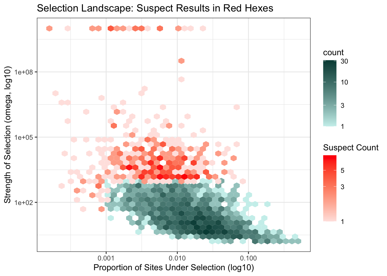
Below we show the hex bin graphs for only the 1:1 Polyneoptera and 1:1 Caelifera selection landscapes.
# Filter for significant genes
parsed_polyneoptera <- busted_SingleStrict %>%
filter(!is.na(padj), padj < 0.05) %>%
filter(!is.na(prop_sites), !is.na(omega3)) %>% # <- ensure both axes are numeric
filter(suspect_result == FALSE)
# Plot
p <- ggplot(parsed_polyneoptera, aes(x = prop_sites, y = omega3)) +
geom_hex(bins = 40) +
scale_fill_gradient(trans = "log10", low = "#ccf0ed", high = "#014a44") +
scale_x_log10() +
scale_y_log10() +
labs(
title = "Selection Landscape for Positively Selected Genes (1:1 Polyneoptera)",
x = "Proportion of Sites Under Selection (log10)",
y = "Strength of Selection (omega, log10)",
fill = "Number of Orthogroups"
) +
theme_bw()
p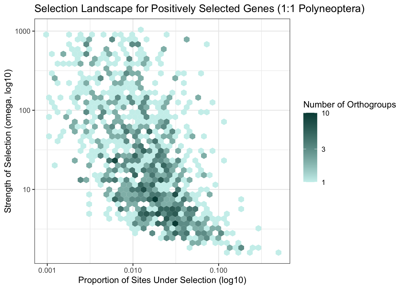
# Filter for significant genes
parsed_locust <- busted_locust %>%
filter(!is.na(padj), padj < 0.05) %>%
filter(!is.na(prop_sites), !is.na(omega3)) %>% # <- ensure both axes are numeric
filter(suspect_result == FALSE)
# We make a hexbin graph only for genes that are locust only
ggplot(parsed_locust, aes(x = prop_sites, y = omega3)) +
geom_hex(bins = 40) +
scale_fill_gradient(trans = "log10", low = "#e6f2ff", high = "#084594") +
scale_x_log10() +
scale_y_log10() +
labs(
title = "Selection on Strict Single-Copy Genes (1:1 Caelifera only)",
x = "Proportion of Sites Under Selection (log10)",
y = "Strength of Selection (omega, log10)",
fill = "Number of Orthogroups"
) +
theme_bw()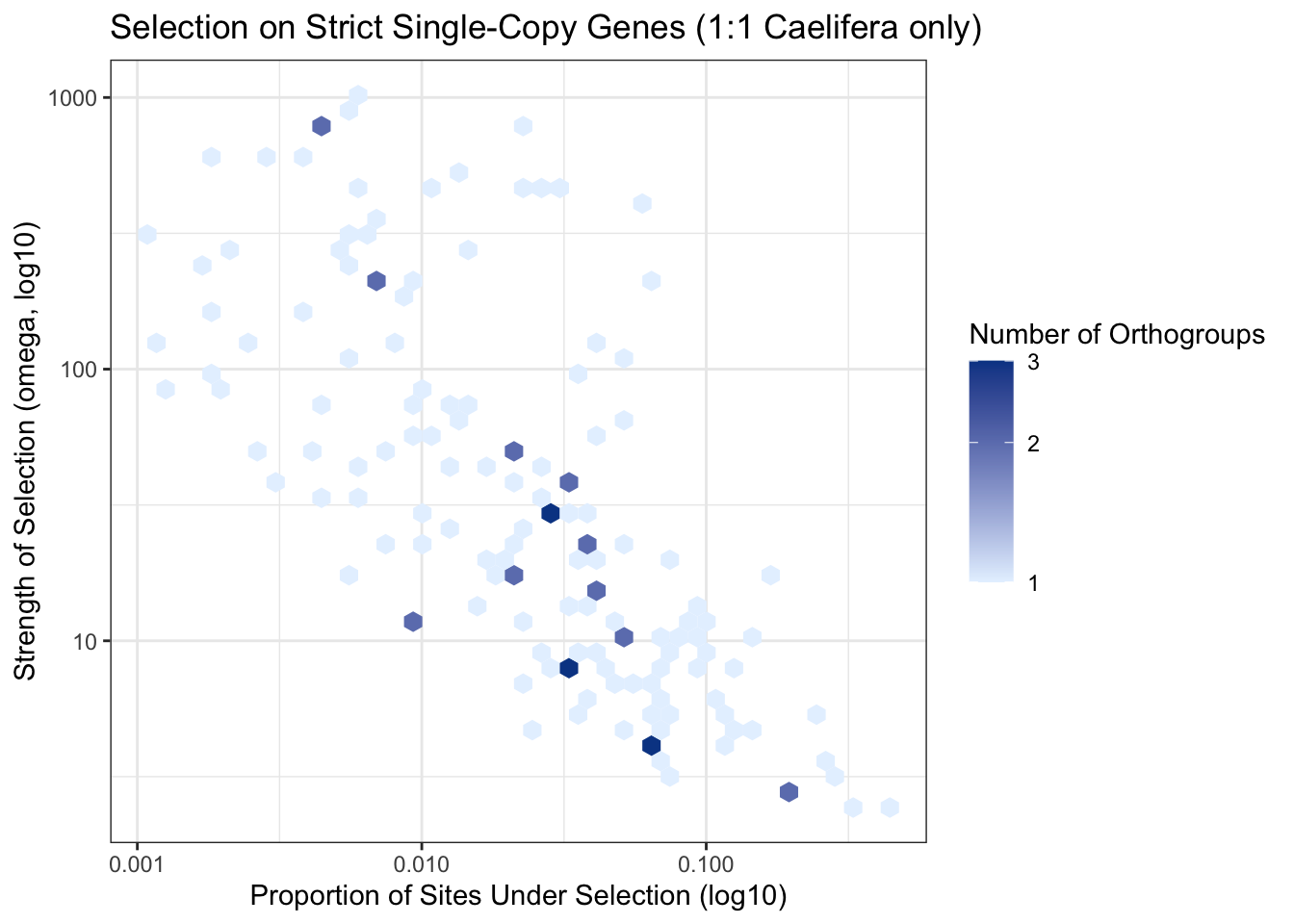
To explore more clearly which orthogroups are showing high selective pressure, we made an interactive version of the hex bin plot below:
library(plotly)
Attaching package: 'plotly'The following object is masked from 'package:XVector':
sliceThe following object is masked from 'package:rtracklayer':
exportThe following object is masked from 'package:AnnotationDbi':
selectThe following object is masked from 'package:IRanges':
sliceThe following object is masked from 'package:S4Vectors':
renameThe following object is masked from 'package:ggplot2':
last_plotThe following object is masked from 'package:stats':
filterThe following object is masked from 'package:graphics':
layout# Prepare your data (already filtered for single-copy, etc.)
plot_data <- parsed_locust %>%
mutate(
log_omega3 = log10(omega3),
log_prop_sites = log10(prop_sites)
)
p <- ggplot(parsed_locust, aes(x = log10(prop_sites), y = log10(omega3))) +
geom_hex(bins = 40, aes(fill = ..count..)) +
geom_point(aes(text = Orthogroup), alpha = 0.1, color = "black") + # invisible overlay for tooltip
scale_fill_viridis_c(trans = "log10") +
labs(
x = "log10(Proportion of Sites Under Selection)",
y = "log10(Omega3)",
fill = "Orthogroup Count",
title = "Interactive Hexbin with Orthogroup Hover (1:1 genes Caelifera only)"
) +
theme_minimal()Warning in geom_point(aes(text = Orthogroup), alpha = 0.1, color = "black"):
Ignoring unknown aesthetics: textggplotly(p, tooltip = "text")Warning: The dot-dot notation (`..count..`) was deprecated in ggplot2 3.4.0.
ℹ Please use `after_stat(count)` instead.
ℹ The deprecated feature was likely used in the ggplot2 package.
Please report the issue at <https://github.com/tidyverse/ggplot2/issues>.
This warning is displayed once per session.
Call `lifecycle::last_lifecycle_warnings()` to see where this warning was
generated.Annotating OGs under selection
Now we will enrich the pathways for which the genes under selection were found:
ortho_dir <- "/Users/maevatecher/Documents/GitHub/locust-comparative-genomics/data/orthofinder/Polyneoptera"
input_file <- file.path(ortho_dir, "Results_I2_iqtree/Orthogroups_genesproteinbiotype_13species_annotated_May2025.csv")
ortho_map <- read.csv(input_file, header = TRUE, stringsAsFactors = FALSE)
head(ortho_map) Orthogroup SpeciesID protein_id GeneID
1 OG0000000 Asimp_filteredTranscripts XP_067003642.2 LOC136874043
2 OG0000000 Asimp_filteredTranscripts XP_067004661.1 LOC136874869
3 OG0000000 Asimp_filteredTranscripts XP_067015293.1 LOC136886419
4 OG0000000 Asimp_filteredTranscripts XP_067015651.2 LOC136886746
5 OG0000000 Asimp_filteredTranscripts XP_068085770.1 LOC137496902
6 OG0000000 Asimp_filteredTranscripts XP_068087037.1 LOC137503369
Description Species GeneType
1 farnesol dehydrogenase isoform X1 Asimp protein-coding
2 dehydrogenase/reductase SDR family member 11 Asimp protein-coding
3 farnesol dehydrogenase Asimp protein-coding
4 farnesol dehydrogenase Asimp protein-coding
5 farnesol dehydrogenase-like Asimp protein-coding
6 farnesol dehydrogenase-like Asimp protein-coding
Accession Begin End Orthogroup_Type
1 NC_090269.1 316521124 316596183 MultiCopy
2 NC_090269.1 316408775 316497937 MultiCopy
3 NC_090279.1 165240845 165292312 MultiCopy
4 NC_090279.1 164532314 164617967 MultiCopy
5 NC_090275.1 60074551 60101839 MultiCopy
6 NC_090279.1 164618824 164719067 MultiCopy# Extract the orthogroup names
selected_orthogroups <- parsed_locust %>%
filter(!is.na(padj), padj < 0.05) %>%
filter(!is.na(prop_sites), !is.na(omega3)) %>% # <- ensure both axes are numeric
filter(suspect_result == FALSE) %>%
pull(Orthogroup) %>% unique()
# Get corresponding GeneID
selected_genes <- ortho_map %>%
filter(Orthogroup %in% selected_orthogroups) %>%
pull(GeneID) %>% unique()We can use the same pipeline and functions as in our section 3: GO enrichment for DEGs.
# === Paths and Constants ===
workDir <- "/Users/maevatecher/Documents/GitHub/locust-comparative-genomics/data"
GODir <- file.path(workDir, "list", "GO_Annotations")
RefDir <- file.path(workDir, "RefSeq")
enrichDir <- file.path(workDir, "HYPHY_selection/functional_pathways/BUSTED_unlabeled")
selListDir <- file.path(workDir, "HYPHY_selection/ParsedBUSTEDResults_unlabeled")
species_list <- c("gregaria", "cancellata", "piceifrons", "americana", "cubense", "nitens")
# === Load Required Libraries ===
library(data.table)
library(dplyr)
library(readr)
library(clusterProfiler)
library(GO.db)
library(rtracklayer)
library(DesertLocustR) # Local installation
gff_map <- c(
gregaria = "GCF_023897955.1_iqSchGreg1.2_genomic.gff",
cancellata = "GCF_023864275.1_iqSchCanc2.1_genomic.gff",
piceifrons = "GCF_021461385.2_iqSchPice1.1_genomic.gff",
americana = "GCF_021461395.2_iqSchAmer2.1_genomic.gff",
cubense = "GCF_023864345.2_iqSchSeri2.2_genomic.gff",
nitens = "GCF_023898315.1_iqSchNite1.1_genomic.gff"
)
annot_map <- c(
gregaria = "EggNog_Arthropoda_one2one.emapper.annotations",
cancellata = "GCF_023864275.1_iqSchCanc2.1_Arthopoda_one2one.emapper.annotations",
piceifrons = "GCF_021461385.2_iqSchPice1.1_Arthopoda_one2one.emapper.annotations",
americana = "GCF_021461395.2_iqSchAmer2.1_Arthopoda_one2one.emapper.annotations",
cubense = "GCF_023864345.2_iqSchSeri2.2_Arthopoda_one2one.emapper.annotations",
nitens = "GCF_023898315.1_iqSchNite1.1_Arthopoda_one2one.emapper.annotations"
)
# GO enrichment
enrich_GO <- function(dge_genes.df, term2gene, term2name, pval, qval){
genes <- rownames(dge_genes.df)
enricher(genes, TERM2GENE = term2gene, TERM2NAME = term2name, pvalueCutoff = pval,
pAdjustMethod = "BH", qvalueCutoff = qval)
}
# KEGG preparation
assign_kegg_ids <- function(sig_genes.df){
if (is.vector(sig_genes.df)) {
sig_genes.df <- data.frame(X.query = sig_genes.df, stringsAsFactors = FALSE)
} else {
sig_genes.df$X.query <- rownames(sig_genes.df)
}
dge_with_kegg_ids <- left_join(sig_genes.df, kegg_final, by = "X.query")
dge_with_kegg_ids$KEGG_ko[grepl("^K", dge_with_kegg_ids$KEGG_ko)]
}
# KEGG enrichment
enrich_KEGG <- function(dge_genes.df, pval_cutoff = 0.05, qval_cutoff = 0.05) {
gene_with_kegg_ids <- assign_kegg_ids(dge_genes.df)
enrichKEGG(
gene = gene_with_kegg_ids,
organism = "ko",
pvalueCutoff = pval_cutoff,
qvalueCutoff = qval_cutoff,
pAdjustMethod = "BH"
)
}
run_GO_enrichment_selected <- function(
gene_list,
go_table,
term2name,
species,
suffix,
ontology,
output_dir,
show_n = 30,
top_n = 30
) {
if (length(gene_list) == 0) return(NULL)
if (!dir.exists(output_dir)) {
dir.create(output_dir, recursive = TRUE)
}
# Make sure column names are correct for clusterProfiler::enricher()
go_table_fixed <- go_table[, 1:2]
colnames(go_table_fixed) <- c("go_id", "gene_id")
term2name_fixed <- term2name[, 1:2]
colnames(term2name_fixed) <- c("go_id", "name")
# Run enrichment
go_result <- enricher(
gene = gene_list,
TERM2GENE = go_table_fixed,
TERM2NAME = term2name_fixed,
pvalueCutoff = 0.05,
qvalueCutoff = 0.05
)
if (!is.null(go_result) &&
inherits(go_result, "enrichResult") &&
nrow(go_result@result) > 0 &&
sum(!is.na(go_result@result$Description)) > 0) {
# Save dotplot
try({
pdf(file = file.path(output_dir, paste0("GO_", ontology, "_dotplot_", species, "_", suffix, ".pdf")),
width = 8, height = 6)
print(dotplot(go_result, showCategory = min(show_n, nrow(go_result@result))) +
ggtitle(paste(ontology, suffix)))
dev.off()
}, silent = TRUE)
# Export top terms with log10(p)
species_enrich_ready <- go_result@result[, c("ID", "p.adjust")]
species_enrich_ready$logp <- -log10(species_enrich_ready$p.adjust)
species_enrich_ready <- species_enrich_ready[order(-species_enrich_ready$logp), ]
species_enrich_ready <- head(species_enrich_ready, n = top_n)[, c("ID", "logp")]
write.table(species_enrich_ready,
file = file.path(output_dir, paste0("enrich_", ontology, "_GOs_", species, "_", suffix, ".txt")),
sep = "\t", quote = FALSE, row.names = FALSE, col.names = FALSE)
# Also export the full table if needed
write.csv(go_result@result,
file = file.path(output_dir, paste0("GO_enrichment_full_", ontology, "_", species, "_", suffix, ".csv")),
row.names = FALSE)
} else {
message(paste0("⚠️ No GO enrichment result to plot/export for ", species, " - ", suffix))
}
}
run_KEGG_enrichment_selected <- function(gene_list, species, suffix, output_dir,
show_n = 40, top_n = 40) {
if (length(gene_list) == 0) return(NULL)
kegg_result <- enrich_KEGG(gene_list, pval_cutoff = 0.05, qval_cutoff = 0.05)
if (!is.null(kegg_result) && inherits(kegg_result, "enrichResult") &&
nrow(kegg_result@result) > 0) {
try({
pdf(file = file.path(output_dir, paste0("KEGG_dotplot_", species, "_", suffix, ".pdf")),
width = 8, height = 6)
print(dotplot(kegg_result, showCategory = min(show_n, nrow(kegg_result@result))) +
ggtitle(paste("KEGG", suffix)))
dev.off()
}, silent = TRUE)
# Full result
write.csv(kegg_result@result,
file = file.path(output_dir, paste0("KEGG_enrichment_", species, "_", suffix, ".csv")),
row.names = FALSE)
# Top KEGG terms
species_enrich_kegg <- kegg_result@result[, c("ID", "p.adjust")]
species_enrich_kegg$logp <- -log10(species_enrich_kegg$p.adjust)
species_enrich_kegg <- species_enrich_kegg[order(-species_enrich_kegg$logp), ][1:min(nrow(species_enrich_kegg), top_n), ]
species_enrich_kegg <- species_enrich_kegg[, c("ID", "logp")]
write.table(species_enrich_kegg,
file = file.path(output_dir, paste0("enrich_KEGG_", species, "_", suffix, ".txt")),
sep = "\t", quote = FALSE, row.names = FALSE, col.names = FALSE)
} else {
message(paste("⚠️ No KEGG enrichment result to plot/export for", species, "-", suffix))
}
}
GO_terms_list <- list()
ontologies_list <- list()
term2name_list <- list()
kegg_final_list <- list()
# Mapping external species names to internal codes in ortho_map
species_translate <- c(
gregaria = "Sgreg",
cancellata = "Scanc",
piceifrons = "Spice",
americana = "Samer", # double-check this is correct
cubense = "Sscub",
nitens = "Snite"
)
for (sp in species_list) {
message("Preparing annotations for ", sp)
sp_code <- species_translate[sp]
eggnog_path <- file.path(GODir, annot_map[[sp]])
gff_path <- file.path(RefDir, gff_map[[sp]])
output_dir <- file.path(enrichDir, sp)
dir.create(output_dir, recursive = TRUE, showWarnings = FALSE)
eggnog_annots <- read.delim(eggnog_path, sep = "\t", skip = 4)
eggnog_annots <- eggnog_annots[1:(nrow(eggnog_annots) - 3), ]
gff.df <- as.data.frame(import(gff_path))
protein_2_gene <- unique(gff.df[c("Name", "gene")])
protein_2_gene_df <- subset(protein_2_gene, grepl("^XP", protein_2_gene$Name))
eggnog_annots$Name <- eggnog_annots$X.query
eggnog_annots <- left_join(eggnog_annots, protein_2_gene_df, by = "Name")
eggnog_annots$X.query <- eggnog_annots$gene
# GO
GO_terms <- data.table(eggnog_annots[, c("X.query", "GOs")])
GO_terms <- GO_terms[, .(GOs = unlist(strsplit(GOs, ","))), by = X.query]
term2name <- GO_terms[, .(GOs, X.query)]
term2name$Names <- mapIds(GO.db, keys = term2name$GOs, column = "TERM", keytype = "GOID")
term2name$Ontology <- mapIds(GO.db, keys = term2name$GOs, column = "ONTOLOGY", keytype = "GOID")
term2name <- as.data.frame(term2name)
go_bp <- term2name[term2name$Ontology == "BP", c("GOs", "X.query")]
go_mf <- term2name[term2name$Ontology == "MF", c("GOs", "X.query")]
go_cc <- term2name[term2name$Ontology == "CC", c("GOs", "X.query")]
term2name_filtered <- term2name[!is.na(term2name$Names), c("GOs", "Names")]
ontologies <- list(BP = go_bp, MF = go_mf, CC = go_cc)
# KEGG
KO_terms <- data.table(eggnog_annots[, c("X.query", "KEGG_ko")])
KO_terms$KEGG_ko <- gsub("ko:", "", KO_terms$KEGG_ko)
KO_terms <- KO_terms[, .(KEGG_ko = unlist(strsplit(KEGG_ko, ","))), by = X.query]
kegg_final <- KO_terms[, .(KEGG_ko, X.query)]
# Store per species
GO_terms_list[[sp]] <- GO_terms
ontologies_list[[sp]] <- ontologies
term2name_list[[sp]] <- term2name_filtered
kegg_final_list[[sp]] <- kegg_final
}Preparing annotations for gregaria'select()' returned 1:1 mapping between keys and columns
'select()' returned 1:1 mapping between keys and columnsPreparing annotations for cancellata'select()' returned 1:1 mapping between keys and columns
'select()' returned 1:1 mapping between keys and columnsPreparing annotations for piceifrons'select()' returned 1:1 mapping between keys and columns
'select()' returned 1:1 mapping between keys and columnsPreparing annotations for americana'select()' returned 1:1 mapping between keys and columns
'select()' returned 1:1 mapping between keys and columnsPreparing annotations for cubense'select()' returned 1:1 mapping between keys and columns
'select()' returned 1:1 mapping between keys and columnsPreparing annotations for nitens'select()' returned 1:1 mapping between keys and columns
'select()' returned 1:1 mapping between keys and columnsFor the Polyneoptera genes: we enrich only for S. gregaria as own model since the genes are orthologs.
# ===== Prepare list of selected genes from orthogroups ====
selected_orthogroups <- parsed_polyneoptera %>%
  filter(!is.na(padj), padj < 0.05) %>%
  filter(!is.na(prop_sites), !is.na(omega3)) %>% # <- ensure both axes are numeric
  filter(suspect_result == FALSE) %>%
  pull(Orthogroup) %>% unique()

selected_genes <- ortho_map %>%
  filter(Orthogroup %in% selected_orthogroups) %>%
  pull(GeneID) %>%
  unique()

# ===== Set up parameters =====
#species_list <- c("gregaria", "cancellata", "piceifrons", "americana", "cubense", "nitens")
species_list <- c("gregaria")
suffix <- "BUSTED_POLYNEOPTERA"

# Mapping external species names to internal codes in ortho_map
species_translate <- c(
  gregaria   = "Sgreg",
  cancellata = "Scanc",
  piceifrons = "Spice",
  americana  = "Samer",  # double-check this is correct
  cubense    = "Sscub",
  nitens     = "Snite"
)

go_results_all <- list()
kegg_results_all <- list()

# ===== Loop through each species =====
for (sp in species_list) {
  message("Processing ", sp)
  sp_code <- species_translate[sp]
  output_dir <- file.path(enrichDir, sp)

  species_genes <- ortho_map %>%
    filter(Orthogroup %in% selected_orthogroups, Species == sp_code) %>%
    pull(GeneID) %>%
    unique()

  # Get species-specific GO terms
  selected_genes_annot <- species_genes[species_genes %in% GO_terms_list[[sp]]$X.query]
  message("→ ", length(selected_genes_annot), " genes for GO enrichment in ", sp)

  # GO enrichment
  go_by_onto <- list()
  for (onto in names(ontologies_list[[sp]])) {
    go_by_onto[[onto]] <- run_GO_enrichment_selected(
      gene_list  = selected_genes_annot,
      go_table   = ontologies_list[[sp]][[onto]],
      term2name  = term2name_list[[sp]],
      species    = sp,
      suffix     = suffix,
      ontology   = onto,
      output_dir = output_dir
    )
  }
  go_results_all[[sp]] <- go_by_onto

  # KEGG enrichment
  kegg_final <<- kegg_final_list[[sp]]  # used inside assign_kegg_ids
  kegg_results_all[[sp]] <- run_KEGG_enrichment_selected(
    gene_list  = selected_genes_annot,
    species    = sp,
    suffix     = suffix,
    output_dir = output_dir
  )
}
Processing gregaria→ 1109 genes for GO enrichment in gregariaNow we check the genes under selection only in Schistocerca clade, only for S. gregaria as own model since the genes are orthologs.
# ===== Prepare list of selected genes from orthogroups =====
selected_orthogroups <- parsed_locust %>%
  filter(!is.na(padj), padj < 0.05) %>%
  filter(!is.na(prop_sites), !is.na(omega3)) %>% # <- ensure both axes are numeric
  filter(suspect_result == FALSE) %>%
  pull(Orthogroup) %>% unique()

selected_genes <- ortho_map %>%
  filter(Orthogroup %in% selected_orthogroups) %>%
  pull(GeneID) %>%
  unique()

# ===== Set up parameters =====
#species_list <- c("gregaria", "cancellata", "piceifrons", "americana", "cubense", "nitens")
species_list <- c("gregaria")
suffix <- "BUSTED_CAELIFERA"

# Mapping external species names to internal codes in ortho_map
species_translate <- c(
  gregaria   = "Sgreg",
  cancellata = "Scanc",
  piceifrons = "Spice",
  americana  = "Samer",  # double-check this is correct
  cubense    = "Sscub",
  nitens     = "Snite"
)

go_results_all <- list()
kegg_results_all <- list()

# ===== Loop through each species =====
for (sp in species_list) {
  message("Processing ", sp)
  sp_code <- species_translate[sp]
  output_dir <- file.path(enrichDir, sp)

  species_genes <- ortho_map %>%
    filter(Orthogroup %in% selected_orthogroups, Species == sp_code) %>%
    pull(GeneID) %>%
    unique()

  # Get species-specific GO terms
  selected_genes_annot <- species_genes[species_genes %in% GO_terms_list[[sp]]$X.query]
  message("→ ", length(selected_genes_annot), " genes for GO enrichment in ", sp)

  # GO enrichment
  go_by_onto <- list()
  for (onto in names(ontologies_list[[sp]])) {
    go_by_onto[[onto]] <- run_GO_enrichment_selected(
      gene_list  = selected_genes_annot,
      go_table   = ontologies_list[[sp]][[onto]],
      term2name  = term2name_list[[sp]],
      species    = sp,
      suffix     = suffix,
      ontology   = onto,
      output_dir = output_dir
    )
  }
  go_results_all[[sp]] <- go_by_onto

  # KEGG enrichment
  kegg_final <<- kegg_final_list[[sp]]  # used inside assign_kegg_ids
  kegg_results_all[[sp]] <- run_KEGG_enrichment_selected(
    gene_list  = selected_genes_annot,
    species    = sp,
    suffix     = suffix,
    output_dir = output_dir
  )
}
Processing gregaria→ 96 genes for GO enrichment in gregariaLabelled
Parsing the json files
To parse the results from the *json files from the BUSTED-PH with
migratory locusts as foreground branches we run this
./scripts/Parsing_BUSTEDresulsr_labelled_June2025.R:
#!/usr/bin/env Rscript

# ============================= #
#         LOAD LIBRARIES       #
# ============================= #
suppressPackageStartupMessages({
  library(tidyverse)
  library(jsonlite)
  library(fs)
})

# ============================= #
#         PARSE ONE FILE       #
# ============================= #
parse_busted <- function(file) {
  tryCatch({
    busted <- jsonlite::fromJSON(file)

    og <- stringr::str_extract(basename(file), "^OG[0-9]+")
    busted_input_file <- busted[["input"]][["file name"]]
    busted_pval <- as.numeric(busted[["test results"]][["p-value"]])

    # Metadata
    aln_length <- busted[["input"]][["number of sites"]]
    seq_count  <- busted[["input"]][["number of sequences"]]

    # Rate model info (Unconstrained model → Test)
    rate_info <- busted[["fits"]][["Unconstrained model"]][["Rate Distributions"]][["Test"]]

    omega_vals <- sapply(rate_info, function(x) as.numeric(x[["omega"]]))
    prop_vals  <- sapply(rate_info, function(x) as.numeric(x[["proportion"]]))

    omega3 <- ifelse(length(omega_vals) >= 3, omega_vals[3], NA)
    prop3  <- ifelse(length(prop_vals) >= 3, prop_vals[3], NA)

    suspect <- is.na(omega3) || omega3 > 1000 || prop3 < 0.001 || aln_length < 100 || seq_count < 4

    tibble(
      file = basename(file),
      input_file = busted_input_file,
      orthogroup = og,
      seq_count = seq_count,
      aln_length = aln_length,
      omega1 = omega_vals[1],
      prop1  = prop_vals[1],
      omega2 = omega_vals[2],
      prop2  = prop_vals[2],
      omega3 = omega3,
      prop_sites = prop3,
      pval = busted_pval,
      padj = p.adjust(busted_pval, method = "BH"),
      significant = p.adjust(busted_pval, method = "BH") < 0.05,
      suspect_result = suspect
    )
  }, error = function(e) {
    message("⚠️ Error parsing: ", file, " → ", e$message)
    return(NULL)
  })
}

# ============================= #
#          RUN SCRIPT          #
# ============================= #

# Define your directories
foreground_dir <- "/Users/maevatecher/Desktop/Polyneoptera_FINAL/8_4_BustedResults_labeled/Locusts/foreground/"
background_dir <- "/Users/maevatecher/Desktop/Polyneoptera_FINAL/8_4_BustedResults_labeled/Locusts/background/"
output_dir     <- "/Users/maevatecher/Desktop/Polyneoptera_FINAL/ParsedBUSTEDResults_labeled"

# Create output folder
dir_create(output_dir)

# Find all files
fg_files <- dir_ls(foreground_dir, glob = "*.json")
bg_files <- dir_ls(background_dir, glob = "*.json")

# Parse all
parsed_fg <- purrr::map_dfr(fg_files, parse_busted) %>% mutate(dataset = "foreground")
parsed_bg <- purrr::map_dfr(bg_files, parse_busted) %>% mutate(dataset = "background")

# Merge
results_all <- bind_rows(parsed_fg, parsed_bg)

# Save
write_csv(results_all, file.path(output_dir, "busted_results_labeled_full.csv"))

message("✅ Parsed labeled BUSTED results for ", nrow(results_all), " genes.")

library(tidyverse)

# Load the parsed results
busted_df <- read_csv("/Users/maevatecher/Desktop/Polyneoptera_FINAL/ParsedBUSTEDResults_labeled/busted_results_labeled_full.csv")

# Pivot all needed columns
busted_summary <- busted_df %>%
  dplyr::select(
    orthogroup, dataset,
    significant, suspect_result,
    seq_count, aln_length,
    omega1, omega2, omega3,
    prop1, prop2, prop_sites,
    pval, padj
  ) %>%
  distinct() %>%
  pivot_wider(
    names_from = dataset,
    values_from = c(
      significant, suspect_result,
      seq_count, aln_length,
      omega1, omega2, omega3,
      prop1, prop2, prop_sites,
      pval, padj
    ),
    names_glue = "{.value}_{dataset}",
    values_fill = NA
  ) %>%
  mutate(
    selection_status = case_when(
      significant_foreground & !significant_background ~ "Foreground only",
      !significant_foreground & significant_background ~ "Background only",
      significant_foreground & significant_background ~ "Both foreground and background",
      TRUE ~ "No selection"
    ),
    suspect_result = suspect_result_foreground | suspect_result_background
  ) %>%
  dplyr::select(
    orthogroup, selection_status, suspect_result,
    pval_foreground, padj_foreground,
    pval_background, padj_background,
    starts_with("seq_count"), starts_with("aln_length"),
    starts_with("omega"), starts_with("prop")
  )

# View or write to file
print(busted_summary)

write_csv(
  busted_summary,
  "/Users/maevatecher/Desktop/Polyneoptera_FINAL/ParsedBUSTEDResults_labeled/busted_orthogroup_summary.csv"
)
Plotting fg vs bg
# ========== Load Libraries ==========
library(tidyverse)

# ========== Load Data ==========
busted_df <- read_csv("/Users/maevatecher/Documents/GitHub/locust-comparative-genomics/data/HYPHY_selection/ParsedBUSTEDResults_labeled/busted_results_labeled_full.csv")
Rows: 10678 Columns: 16
── Column specification ────────────────────────────────────────────────────────
Delimiter: ","
chr (4): file, input_file, orthogroup, dataset
dbl (10): seq_count, aln_length, omega1, prop1, omega2, prop2, omega3, prop_...
lgl (2): significant, suspect_result
ℹ Use `spec()` to retrieve the full column specification for this data.
ℹ Specify the column types or set `show_col_types = FALSE` to quiet this message.# ========== Data Preparation ==========
# Pivot to wide format
plot_df <- busted_df %>%
dplyr::select(orthogroup, dataset, omega3, significant, suspect_result) %>%
pivot_wider(
names_from = dataset,
values_from = c(omega3, significant, suspect_result),
names_sep = "_"
) %>%
# Filter out rows with missing omega3 or suspect results
filter(
!is.na(omega3_foreground),
!is.na(omega3_background),
suspect_result_foreground == FALSE,
suspect_result_background == FALSE
) %>%
# Log-transform omega3
mutate(
log_omega3_fore = log10(omega3_foreground + 1e-3),
log_omega3_back = log10(omega3_background + 1e-3),
color_status = case_when(
significant_foreground ~ "Positive Selection",
TRUE ~ "Not Significant"
)
)
# ========== Plot ==========
plot <- ggplot(plot_df, aes(x = log_omega3_fore, y = log_omega3_back)) +
geom_point(aes(color = color_status), size = 3, alpha = 0.8) +
scale_color_manual(values = c("Positive Selection" = "#9B59B6", "Not Significant" = "gray80")) +
labs(
x = expression(log[10]~omega[3]~"(foreground branches)"),
y = expression(log[10]~omega[3]~"(background branches)"),
color = "Selection"
) +
coord_cartesian(xlim = c(-2, 4), ylim = c(-2, 4)) +
theme_minimal(base_size = 14) +
theme(legend.position = "top")
# ========== Export ==========
ggsave("bustedPH_logomega3_scatter_nosuspect.pdf", plot, width = 8, height = 6)
# Preview
print(plot)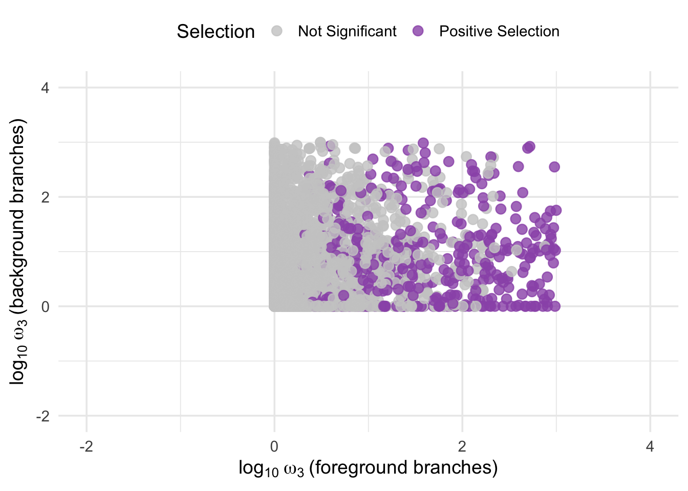
| Version | Author | Date |
|---|---|---|
| 6e321f0 | Maeva TECHER | 2026-04-06 |
Labelled Pruned
Parsing the json files
#!/usr/bin/env Rscript

# ============================= #
#         LOAD LIBRARIES       #
# ============================= #
suppressPackageStartupMessages({
  library(tidyverse)
  library(jsonlite)
  library(fs)
})

# ============================= #
#         PARSE ONE FILE       #
# ============================= #
parse_busted <- function(file) {
  tryCatch({
    busted <- jsonlite::fromJSON(file)

    og <- stringr::str_extract(basename(file), "^OG[0-9]+")
    busted_input_file <- busted[["input"]][["file name"]]
    busted_pval <- as.numeric(busted[["test results"]][["p-value"]])

    # Metadata
    aln_length <- busted[["input"]][["number of sites"]]
    seq_count  <- busted[["input"]][["number of sequences"]]

    # Rate model info (Unconstrained model → Test)
    rate_info <- busted[["fits"]][["Unconstrained model"]][["Rate Distributions"]][["Test"]]

    omega_vals <- sapply(rate_info, function(x) as.numeric(x[["omega"]]))
    prop_vals  <- sapply(rate_info, function(x) as.numeric(x[["proportion"]]))

    omega3 <- ifelse(length(omega_vals) >= 3, omega_vals[3], NA)
    prop3  <- ifelse(length(prop_vals) >= 3, prop_vals[3], NA)

    suspect <- is.na(omega3) || omega3 > 1000 || prop3 < 0.001 || aln_length < 100 || seq_count < 4

    tibble(
      file = basename(file),
      input_file = busted_input_file,
      orthogroup = og,
      seq_count = seq_count,
      aln_length = aln_length,
      omega1 = omega_vals[1],
      prop1  = prop_vals[1],
      omega2 = omega_vals[2],
      prop2  = prop_vals[2],
      omega3 = omega3,
      prop_sites = prop3,
      pval = busted_pval,
      padj = p.adjust(busted_pval, method = "BH"),
      significant = p.adjust(busted_pval, method = "BH") < 0.05,
      suspect_result = suspect
    )
  }, error = function(e) {
    message("⚠️ Error parsing: ", file, " → ", e$message)
    return(NULL)
  })
}

# ============================= #
#          RUN SCRIPT          #
# ============================= #

# Define your directories
foreground_dir <- "/Users/maevatecher/Desktop/Polyneoptera_FINAL/8_4_BustedResults_labeled_Pruned/Locusts/foreground/"
background_dir <- "/Users/maevatecher/Desktop/Polyneoptera_FINAL/8_4_BustedResults_labeled_Pruned/Locusts/background/"
output_dir     <- "/Users/maevatecher/Desktop/Polyneoptera_FINAL/ParsedBUSTEDResults_labeled_Pruned"

# Create output folder
dir_create(output_dir)

# Find all files
fg_files <- dir_ls(foreground_dir, glob = "*.json")
bg_files <- dir_ls(background_dir, glob = "*.json")

# Parse all
parsed_fg <- purrr::map_dfr(fg_files, parse_busted) %>% mutate(dataset = "foreground")
parsed_bg <- purrr::map_dfr(bg_files, parse_busted) %>% mutate(dataset = "background")

# Merge
results_all <- bind_rows(parsed_fg, parsed_bg)

# Save
write_csv(results_all, file.path(output_dir, "busted_results_labeled_full.csv"))

message("✅ Parsed labeled BUSTED results for ", nrow(results_all), " genes.")

library(tidyverse)

# Load the parsed results
busted_df <- read_csv("/Users/maevatecher/Desktop/Polyneoptera_FINAL/ParsedBUSTEDResults_labeled_Pruned/busted_results_labeled_full.csv")

# Pivot all needed columns
busted_summary <- busted_df %>%
  dplyr::select(
    orthogroup, dataset,
    significant, suspect_result,
    seq_count, aln_length,
    omega1, omega2, omega3,
    prop1, prop2, prop_sites,
    pval, padj
  ) %>%
  distinct() %>%
  pivot_wider(
    names_from = dataset,
    values_from = c(
      significant, suspect_result,
      seq_count, aln_length,
      omega1, omega2, omega3,
      prop1, prop2, prop_sites,
      pval, padj
    ),
    names_glue = "{.value}_{dataset}",
    values_fill = NA
  ) %>%
  mutate(
    selection_status = case_when(
      significant_foreground & !significant_background ~ "Foreground only",
      !significant_foreground & significant_background ~ "Background only",
      significant_foreground & significant_background ~ "Both foreground and background",
      TRUE ~ "No selection"
    ),
    suspect_result = suspect_result_foreground | suspect_result_background
  ) %>%
  dplyr::select(
    orthogroup, selection_status, suspect_result,
    pval_foreground, padj_foreground,
    pval_background, padj_background,
    starts_with("seq_count"), starts_with("aln_length"),
    starts_with("omega"), starts_with("prop")
  )

# View or write to file
print(busted_summary)

write_csv(
  busted_summary,
  "/Users/maevatecher/Desktop/Polyneoptera_FINAL/ParsedBUSTEDResults_labeled_Pruned/busted_orthogroup_summary.csv"
)
Plotting fg vs bg
# ========== Load Libraries ==========
library(tidyverse)

# ========== Load Data ==========
busted_df <- read_csv("/Users/maevatecher/Documents/GitHub/locust-comparative-genomics/data/HYPHY_selection/ParsedBUSTEDResults_labeled_Pruned/busted_results_labeled_full.csv")
Rows: 10676 Columns: 16
── Column specification ────────────────────────────────────────────────────────
Delimiter: ","
chr (4): file, input_file, orthogroup, dataset
dbl (10): seq_count, aln_length, omega1, prop1, omega2, prop2, omega3, prop_...
lgl (2): significant, suspect_result
ℹ Use `spec()` to retrieve the full column specification for this data.
ℹ Specify the column types or set `show_col_types = FALSE` to quiet this message.# ========== Data Preparation ==========
# Pivot to wide format
plot_df <- busted_df %>%
dplyr::select(orthogroup, dataset, omega3, significant, suspect_result) %>%
pivot_wider(
names_from = dataset,
values_from = c(omega3, significant, suspect_result),
names_sep = "_"
) %>%
# Filter out rows with missing omega3 or suspect results
filter(
!is.na(omega3_foreground),
!is.na(omega3_background),
suspect_result_foreground == FALSE,
suspect_result_background == FALSE
) %>%
# Log-transform omega3
mutate(
log_omega3_fore = log10(omega3_foreground + 1e-3),
log_omega3_back = log10(omega3_background + 1e-3),
color_status = case_when(
significant_foreground ~ "Positive Selection",
TRUE ~ "Not Significant"
)
)
# ========== Plot ==========
plot <- ggplot(plot_df, aes(x = log_omega3_fore, y = log_omega3_back)) +
geom_point(aes(color = color_status), size = 3, alpha = 0.8) +
scale_color_manual(values = c("Positive Selection" = "#9B59B6", "Not Significant" = "gray80")) +
labs(
x = expression(log[10]~omega[3]~"(foreground branches)"),
y = expression(log[10]~omega[3]~"(background branches)"),
color = "Selection"
) +
coord_cartesian(xlim = c(-2, 4), ylim = c(-2, 4)) +
theme_minimal(base_size = 14) +
theme(legend.position = "top")
# ========== Export ==========
ggsave("bustedPH_logomega3_scatter_nosuspect.pdf", plot, width = 8, height = 6)
# Preview
print(plot)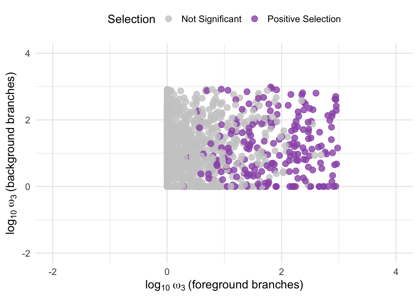
| Version | Author | Date |
|---|---|---|
| 6e321f0 | Maeva TECHER | 2026-04-06 |
9. RELAX
Running the analysis
We will perform RELAX analysis to check whether the foreground branches that have experienced selection were intensifying or relaxing:
# For Polyneoptera

# For labelled phylogeny
sbatch ./scripts/RunRELAX_labeled_May2025.sh \
/scratch/group/songlab/maeva/LocustsGenomeEvolution/Polyneoptera_FINAL/9_1_LabelledPhylogenies/Locusts \
Locusts \
/scratch/group/songlab/maeva/LocustsGenomeEvolution/Polyneoptera_FINAL/5_OrthoFinder/fasta/Results_May26_iqtree/Orthogroups/Orthogroups_SingleCopyOrthologues_selanalysiswide.txt

# For labelled phylogeny PRUNED
sbatch ./scripts/RunRELAX_labeled_June2025.sh \
/scratch/group/songlab/maeva/LocustsGenomeEvolution/Polyneoptera_FINAL/9_1_LabelledPhylogenies_Pruned/Locusts \
Locusts \
/scratch/group/songlab/maeva/LocustsGenomeEvolution/Polyneoptera_FINAL/5_OrthoFinder/fasta/Results_May26_iqtree/Orthogroups/Orthogroups_SingleCopyOrthologues_selanalysiswide.txt
Labelled
Parsing the json files
For parsing the results, you just do:
# ============ SETTINGS ============
input_dir <- "/Users/maevatecher/Desktop/Polyneoptera_FINAL/10_1_RelaxResults"
single_copy_file <- "/Users/maevatecher/Documents/GitHub/locust-comparative-genomics/data/orthofinder/Polyneoptera/Results_I2_iqtree/Orthogroups/Orthogroups_SingleCopyOrthologues_selanalysiswide.txt"
output_dir <- "/Users/maevatecher/Desktop/Polyneoptera_FINAL/ParsedRELAXResults"
dir.create(output_dir, showWarnings = FALSE, recursive = TRUE)

# ============ LIBRARIES ============
library(jsonlite)
library(tidyverse)

# ============ FUNCTIONS ============
parse_relax_json <- function(file) {
  tryCatch({
    result <- fromJSON(file)

    og <- stringr::str_extract(basename(file), "^OG[0-9]+")
    input_file <- result[["input"]][["file name"]]
    seq_count <- result[["input"]][["number of sequences"]]
    aln_length <- result[["input"]][["number of sites"]]

    test_results <- result[["test results"]]

    pval <- as.numeric(test_results[["p-value"]])
    k_val <- as.numeric(test_results[["relaxation or intensification parameter"]])

    selection_type <- case_when(
      is.na(pval) ~ "Undetermined",
      pval < 0.05 & k_val > 1 ~ "Intensification",
      pval < 0.05 & k_val < 1 ~ "Relaxation",
      TRUE ~ "No significant difference"
    )

    suspect <- is.na(k_val) || k_val > 10 || k_val < 0.1 || is.na(pval) || aln_length < 100 || seq_count < 4

    tibble(
      file = file,
      input_file = input_file,
      orthogroup = og,
      seq_count = seq_count,
      aln_length = aln_length,
      k = k_val,
      pval = pval,
      padj = NA,  # placeholder, will be set after all parsing
      selection_type = selection_type,
      suspect_result = suspect
    )
  }, error = function(e) {
    message("⚠️ Error parsing ", file, ": ", e$message)
    return(NULL)
  })
}

relax_results <- parse_all_relax_jsons(input_dir)

if (nrow(relax_results) > 0) {
  relax_results <- relax_results %>%
    mutate(
      padj = p.adjust(pval, method = "BH"),
      significant = padj < 0.05
    )
}

parse_all_relax_jsons <- function(folder) {
  files <- list.files(folder, pattern = "\\.json$", full.names = TRUE)
  files <- files[file.info(files)$size > 0]

  results <- purrr::map_dfr(files, parse_relax_json)

  results <- results %>%
    mutate(
      padj = p.adjust(pval, method = "BH"),
      significant = padj < 0.05
    )

  return(results)
}

# ============ EXECUTE PARSING ============
relax_results <- parse_all_relax_jsons(input_dir)

# ============ WRITE OUTPUT ============
write_csv(relax_results, file.path(output_dir, "relax_results.csv"))
message("✅ Parsed RELAX results saved to: ", file.path(output_dir, "relax_results_csv"))
Combined results
# Load required libraries
library(readr)
library(dplyr)

# === Define file paths ===
busted_file <- "/Users/maevatecher/Documents/GitHub/locust-comparative-genomics/data/HYPHY_selection/ParsedBUSTEDResults_labeled/busted_orthogroup_summary.csv"
relax_file  <- "/Users/maevatecher/Documents/GitHub/locust-comparative-genomics/data/HYPHY_selection/ParsedRELAXResults/relax_results.csv"

# === Read in both tables ===
busted_df <- read_csv(busted_file, show_col_types = FALSE)
relax_df  <- read_csv(relax_file, show_col_types = FALSE)

# === Left join BUSTED + RELAX results ===
combined_df <- left_join(busted_df, relax_df, by = "orthogroup")

# === Preview and save ===
head(combined_df)
# A tibble: 6 × 33
orthogroup selection_status suspect_result.x pval_foreground padj_foreground
<chr> <chr> <lgl> <dbl> <dbl>
1 OG0004339 Background only FALSE 0.5 0.5
2 OG0004340 Background only FALSE 0.0744 0.0744
3 OG0004341 Foreground only TRUE 0.0000166 0.0000166
4 OG0004343 No selection FALSE 0.487 0.487
5 OG0004344 No selection TRUE 0.5 0.5
6 OG0004345 No selection FALSE 0.161 0.161
# ℹ 28 more variables: pval_background <dbl>, padj_background <dbl>,
# seq_count_foreground <dbl>, seq_count_background <dbl>,
# aln_length_foreground <dbl>, aln_length_background <dbl>,
# omega1_foreground <dbl>, omega1_background <dbl>, omega2_foreground <dbl>,
# omega2_background <dbl>, omega3_foreground <dbl>, omega3_background <dbl>,
# prop1_foreground <dbl>, prop1_background <dbl>, prop2_foreground <dbl>,
# prop2_background <dbl>, prop_sites_foreground <dbl>, …# Save combined table
write_csv(combined_df, "/Users/maevatecher/Documents/GitHub/locust-comparative-genomics/data/HYPHY_selection/ParsedRELAXResults/joint_busted_relax_results.csv")
message("✅ Combined BUSTED + RELAX table saved.")✅ Combined BUSTED + RELAX table saved.Labelled pruned
Parsing the json files
For parsing the results, you just do:
# ============ SETTINGS ============
input_dir <- "/Users/maevatecher/Desktop/Polyneoptera_FINAL/10_1_RelaxResults_Pruned"
single_copy_file <- "/Users/maevatecher/Documents/GitHub/locust-comparative-genomics/data/orthofinder/Polyneoptera/Results_I2_iqtree/Orthogroups/Orthogroups_SingleCopyOrthologues_selanalysiswide.txt"
output_dir <- "/Users/maevatecher/Desktop/Polyneoptera_FINAL/ParsedRELAXResults_Pruned"
dir.create(output_dir, showWarnings = FALSE, recursive = TRUE)

# ============ LIBRARIES ============
library(jsonlite)
library(tidyverse)

# ============ FUNCTIONS ============
parse_relax_json <- function(file) {
  tryCatch({
    result <- fromJSON(file)

    og <- stringr::str_extract(basename(file), "^OG[0-9]+")
    input_file <- result[["input"]][["file name"]]
    seq_count <- result[["input"]][["number of sequences"]]
    aln_length <- result[["input"]][["number of sites"]]

    test_results <- result[["test results"]]

    pval <- as.numeric(test_results[["p-value"]])
    k_val <- as.numeric(test_results[["relaxation or intensification parameter"]])

    selection_type <- case_when(
      is.na(pval) ~ "Undetermined",
      pval < 0.05 & k_val > 1 ~ "Intensification",
      pval < 0.05 & k_val < 1 ~ "Relaxation",
      TRUE ~ "No significant difference"
    )

    suspect <- is.na(k_val) || k_val > 10 || k_val < 0.1 || is.na(pval) || aln_length < 100 || seq_count < 4

    tibble(
      file = file,
      input_file = input_file,
      orthogroup = og,
      seq_count = seq_count,
      aln_length = aln_length,
      k = k_val,
      pval = pval,
      padj = NA,  # placeholder, will be set after all parsing
      selection_type = selection_type,
      suspect_result = suspect
    )
  }, error = function(e) {
    message("⚠️ Error parsing ", file, ": ", e$message)
    return(NULL)
  })
}

relax_results <- parse_all_relax_jsons(input_dir)

if (nrow(relax_results) > 0) {
  relax_results <- relax_results %>%
    mutate(
      padj = p.adjust(pval, method = "BH"),
      significant = padj < 0.05
    )
}

parse_all_relax_jsons <- function(folder) {
  files <- list.files(folder, pattern = "\\.json$", full.names = TRUE)
  files <- files[file.info(files)$size > 0]

  results <- purrr::map_dfr(files, parse_relax_json)

  results <- results %>%
    mutate(
      padj = p.adjust(pval, method = "BH"),
      significant = padj < 0.05
    )

  return(results)
}

# ============ EXECUTE PARSING ============
relax_results <- parse_all_relax_jsons(input_dir)

# ============ WRITE OUTPUT ============
write_csv(relax_results, file.path(output_dir, "relax_results.csv"))
message("✅ Parsed RELAX results saved to: ", file.path(output_dir, "relax_results_csv"))
Warning: The above code chunk cached its results, but
it won’t be re-run if previous chunks it depends on are updated. If you
need to use caching, it is highly recommended to also set
knitr::opts_chunk$set(autodep = TRUE) at the top of the
file (in a chunk that is not cached). Alternatively, you can customize
the option dependson for each individual chunk that is
cached. Using either autodep or dependson will
remove this warning. See the
knitr cache options for more details.
Combined results
# Load required libraries
library(readr)
library(dplyr)

# === Define file paths ===
busted_file <- "/Users/maevatecher/Documents/GitHub/locust-comparative-genomics/data/HYPHY_selection/ParsedBUSTEDResults_labeled_Pruned/busted_orthogroup_summary.csv"
relax_file  <- "/Users/maevatecher/Documents/GitHub/locust-comparative-genomics/data/HYPHY_selection/ParsedRELAXResults_Pruned/relax_results.csv"

# === Read in both tables ===
busted_df <- read_csv(busted_file, show_col_types = FALSE)
relax_df  <- read_csv(relax_file, show_col_types = FALSE)

# === Left join BUSTED + RELAX results ===
combined_df <- left_join(busted_df, relax_df, by = "orthogroup")

# === Preview and save ===
head(combined_df)
# A tibble: 6 × 33
orthogroup selection_status suspect_result.x pval_foreground padj_foreground
<chr> <chr> <lgl> <dbl> <dbl>
1 OG0004339 No selection TRUE 0.5 0.5
2 OG0004340 Background only FALSE 0.188 0.188
3 OG0004341 Foreground only TRUE 0.0000218 0.0000218
4 OG0004343 No selection FALSE 0.0943 0.0943
5 OG0004344 No selection TRUE 0.114 0.114
6 OG0004345 Foreground only FALSE 0.0378 0.0378
# ℹ 28 more variables: pval_background <dbl>, padj_background <dbl>,
# seq_count_foreground <dbl>, seq_count_background <dbl>,
# aln_length_foreground <dbl>, aln_length_background <dbl>,
# omega1_foreground <dbl>, omega1_background <dbl>, omega2_foreground <dbl>,
# omega2_background <dbl>, omega3_foreground <dbl>, omega3_background <dbl>,
# prop1_foreground <dbl>, prop1_background <dbl>, prop2_foreground <dbl>,
# prop2_background <dbl>, prop_sites_foreground <dbl>, …# Save combined table
write_csv(combined_df, "/Users/maevatecher/Documents/GitHub/locust-comparative-genomics/data/HYPHY_selection/ParsedRELAXResults_Pruned/joint_busted_relax_results.csv")
message("✅ Combined BUSTED + RELAX table saved.")✅ Combined BUSTED + RELAX table saved.10. Combined BUSTED and RELAX
Full tree
# Load libraries
library(readr)
library(dplyr)
library(ComplexUpset)
library(ggplot2)

# Load your dataset
df <- read_csv("/Users/maevatecher/Documents/GitHub/locust-comparative-genomics/data/HYPHY_selection/ParsedRELAXResults/joint_busted_relax_annotated.csv", show_col_types = FALSE)

# Recalculate selection_type from k and pval
df <- df %>%
  mutate(
    k_val = as.numeric(k),
    pval = as.numeric(pval),
    padj = as.numeric(padj),
    selection_type = case_when(
      is.na(pval) ~ "Undetermined",
      pval < 0.05 & k_val > 1 ~ "Intensification",
      pval < 0.05 & k_val < 1 ~ "Relaxation",
      TRUE ~ "No significant difference"
    )
  )

# Filter non-suspect orthogroups
df_suspect <- df %>%
  filter(selection_status != "No selection") %>%
  filter(suspect_result.x == FALSE) %>%
  mutate(
    PSG = selection_status %in% c("Foreground only", "Both foreground and background"),
    Relaxation = selection_type == "Relaxation",
    Intensification = selection_type == "Intensification",
    Insignificant = selection_type == "No significant difference"
  ) %>%
  dplyr::select(orthogroup, PSG, Relaxation, Intensification, Insignificant) %>%
  distinct()

# Add color groups: PSG > Relaxation > Other
df_suspect <- df_suspect %>%
  mutate(
    PSG_color = case_when(
      PSG ~ "PSG",
      Relaxation ~ "Relaxation",
      Intensification ~ "Intensification",
      TRUE ~ "Other"
    )
  )

# Define color palette
custom_colors <- c(
  "PSG" = "orchid",         # Green
  "Relaxation" = "gold",   # Orange
  "Intensification" = "tomato",   # Orange
  "Other" = "black"         # Default gray
)


# Reorder factor levels BEFORE calling upset()
df_suspect_long <- df_suspect %>%
  pivot_longer(cols = c("PSG", "Relaxation", "Intensification", "Insignificant"),
               names_to = "set", values_to = "value") %>%
  filter(value) %>%
  mutate(set = factor(set, levels = c("Insignificant",  "Intensification", "Relaxation", "PSG"))) %>%
  pivot_wider(names_from = set, values_from = value, values_fill = FALSE)

# Add color groups again
df_suspect_long <- df_suspect_long %>%
  mutate(
    PSG_color = case_when(
      PSG ~ "PSG",
      Relaxation ~ "Relaxation",
      Intensification ~ "Intensification",
      TRUE ~ "Other"
    )
  )


busted_summary <- df %>%
  filter(suspect_result.x == FALSE) %>%
  distinct(orthogroup, selection_status) %>%
  mutate(
    selection_status = factor(
      selection_status,
      levels = c(
        "Foreground only",
        "Background only",
        "Both foreground and background",
        "No selection"
      )
    )
  ) %>%
  count(selection_status, name = "n_orthogroups") %>%
  mutate(
    total_tested = sum(n_orthogroups),
    percent = round(100 * n_orthogroups / total_tested, 2)
  )

print(busted_summary)
# A tibble: 4 × 4
selection_status n_orthogroups total_tested percent
<fct> <int> <int> <dbl>
1 Foreground only 233 2604 8.95
2 Background only 895 2604 34.4
3 Both foreground and background 196 2604 7.53
4 No selection 1280 2604 49.2 #ComplexUpset::upset(
# df_suspect_long,
# intersect = c("Insignificant", "Intensification", "Relaxation", "PSG"),
# name = "Selection Category",
# sort_sets = FALSE,
# sort_intersections = FALSE,
# intersections=list(
# c('PSG', 'Relaxation'),
# c('PSG', 'Intensification'),
# c('PSG', 'Insignificant'),
# 'Relaxation',
# 'Intensification',
# 'Insignificant'
# ),
# sort_intersections_by = "degree",
# set_sizes = upset_set_size() +
# ggtitle("Set Size") +
# theme_minimal(),
# base_annotations = list(
# 'Intersection size' = intersection_size(
# mapping = aes(fill = PSG_color),
# text = list(size = 3),
# bar_number_threshold = 10
# ) +
# scale_fill_manual(values = custom_colors, guide = "none")
# ),
# queries=list(
# upset_query(
# intersect=c('PSG', 'Relaxation'),
# color='orchid',
# fill='orchid',
# only_components=c('intersections_matrix', 'Intersection size')
# ),
# upset_query(
# intersect=c('PSG', 'Intensification'),
# color='orchid',
# fill='orchid',
# only_components=c('intersections_matrix', 'Intersection size')
# ),
# upset_query(
# intersect=c('PSG', 'Insignificant'),
# color='orchid',
# fill='orchid',
# only_components=c('intersections_matrix', 'Intersection size')
# ),
# upset_query(
# intersect=c('Relaxation'),
# color='gold',
# fill='gold',
# only_components=c('intersections_matrix', 'Intersection size')
# ),
# upset_query(
# intersect=c('Intensification'),
# color='tomato',
# fill='tomato',
# only_components=c('intersections_matrix', 'Intersection size')
# ),
# upset_query(set='PSG', fill='orchid'),
# upset_query(set='Relaxation', fill='gold'),
# upset_query(set='Intensification', fill='tomato'),
# upset_query(set='Insignificant', fill='black')
# )) +
# ggtitle("Genes under positive selection in swarming species (Full tree)") +
# theme_minimal(base_size = 12)
library(readr)
library(dplyr)
library(ggplot2)
library(patchwork)
# Load dataset
df <- read_csv(
"/Users/maevatecher/Documents/GitHub/locust-comparative-genomics/data/HYPHY_selection/ParsedRELAXResults/joint_busted_relax_annotated.csv",
show_col_types = FALSE
)
# Recalculate selection_type from k and pval
df <- df %>%
mutate(
k_val = as.numeric(k),
pval = as.numeric(pval),
padj = as.numeric(padj),
selection_type = case_when(
is.na(pval) ~ "Undetermined",
pval < 0.05 & k_val > 1 ~ "Intensification",
pval < 0.05 & k_val < 1 ~ "Relaxation",
TRUE ~ "No significant difference"
)
)
# -----------------------------
# Plot 1: BUSTED-PH categories
# -----------------------------
busted_summary <- df %>%
filter(suspect_result.x == FALSE) %>%
distinct(orthogroup, selection_status) %>%
mutate(
selection_status = case_when(
selection_status == "Foreground only" ~ "Foreground only",
selection_status == "Background only" ~ "Background only",
selection_status == "Both foreground and background" ~ "Both",
TRUE ~ "No selection"
)
) %>%
count(selection_status, name = "n") %>%
mutate(
selection_status = factor(
selection_status,
levels = c("Foreground only", "Background only", "Both", "No selection")
)
)
plot_busted <- ggplot(
busted_summary,
aes(x = selection_status, y = n, fill = selection_status)
) +
geom_col(width = 0.7, color = "black", linewidth = 0.2) +
geom_text(aes(label = n), vjust = -0.3, fontface = "bold", size = 4) +
scale_fill_manual(values = c(
"Foreground only" = "orchid",
"Background only" = "gray60",
"Both" = "tomato",
"No selection" = "gray90"
)) +
labs(
title = "BUSTED-PH",
subtitle = "Orthogroups tested",
x = NULL,
y = "Orthogroups"
) +
theme_minimal(base_size = 12) +
theme(
legend.position = "none",
plot.title = element_text(face = "bold", hjust = 0.5),
plot.subtitle = element_text(hjust = 0.5),
axis.text.x = element_text(face = "bold", angle = 20, hjust = 1)
)
# -----------------------------
# RELAX summary function
# -----------------------------
make_relax_summary <- function(data, status_label, panel_label) {
data %>%
filter(suspect_result.x == FALSE) %>%
distinct(orthogroup, selection_status, selection_type) %>%
filter(selection_status == status_label) %>%
mutate(
selection_type = case_when(
selection_type == "Intensification" ~ "Intensification",
selection_type == "Relaxation" ~ "Relaxation",
TRUE ~ "No significant difference"
),
selection_type = factor(
selection_type,
levels = c("Intensification", "Relaxation", "No significant difference")
),
panel = panel_label
) %>%
count(panel, selection_type, name = "n")
}
# Build foreground/background RELAX summaries
relax_summary_bg <- make_relax_summary(df, "Background only", "Background-only")
relax_summary_fg <- make_relax_summary(df, "Foreground only", "Foreground-only")
# Shared y limit for both RELAX panels
relax_ymax <- max(c(relax_summary_bg$n, relax_summary_fg$n), na.rm = TRUE) * 1.15
# -----------------------------
# Plot 2A: RELAX background-only
# -----------------------------
plot_relax_bg <- ggplot(
relax_summary_bg,
aes(x = selection_type, y = n, fill = selection_type)
) +
geom_col(width = 0.7, color = "black", linewidth = 0.2) +
geom_text(aes(label = n), vjust = -0.3, fontface = "bold", size = 4) +
scale_fill_manual(values = c(
"Intensification" = "tomato",
"Relaxation" = "gold",
"No significant difference" = "black"
)) +
coord_cartesian(ylim = c(0, relax_ymax)) +
labs(
title = "RELAX",
subtitle = "Background-only",
x = NULL,
y = "Orthogroups"
) +
theme_minimal(base_size = 12) +
theme(
legend.position = "none",
plot.title = element_text(face = "bold", hjust = 0.5),
plot.subtitle = element_text(hjust = 0.5),
axis.text.x = element_blank(),
axis.ticks.x = element_blank()
)
# -----------------------------
# Plot 2B: RELAX foreground-only
# -----------------------------
plot_relax_fg <- ggplot(
relax_summary_fg,
aes(x = selection_type, y = n, fill = selection_type)
) +
geom_col(width = 0.7, color = "black", linewidth = 0.2) +
geom_text(aes(label = n), vjust = -0.3, fontface = "bold", size = 4) +
scale_fill_manual(values = c(
"Intensification" = "tomato",
"Relaxation" = "gold",
"No significant difference" = "black"
)) +
coord_cartesian(ylim = c(0, relax_ymax)) +
labs(
title = NULL,
subtitle = "Foreground-only",
x = NULL,
y = "Orthogroups"
) +
theme_minimal(base_size = 12) +
theme(
legend.position = "none",
plot.subtitle = element_text(hjust = 0.5),
axis.text.x = element_text(face = "bold", angle = 20, hjust = 1)
)
# -----------------------------
# Combine layout
# -----------------------------
final_plot <- plot_busted | (plot_relax_bg / plot_relax_fg)
final_plot
Pruned tree
# Load libraries
library(readr)
library(dplyr)
library(ComplexUpset)
library(ggplot2)

# Load your dataset
df <- read_csv("/Users/maevatecher/Documents/GitHub/locust-comparative-genomics/data/HYPHY_selection/ParsedRELAXResults_Pruned/joint_busted_relax_annotated.csv", show_col_types = FALSE)

# Recalculate selection_type from k and pval
df <- df %>%
  mutate(
    k_val = as.numeric(k),
    pval = as.numeric(pval),
    padj = as.numeric(padj),
    selection_type = case_when(
      is.na(pval) ~ "Undetermined",
      pval < 0.05 & k_val > 1 ~ "Intensification",
      pval < 0.05 & k_val < 1 ~ "Relaxation",
      TRUE ~ "No significant difference"
    )
  )

# Filter non-suspect orthogroups
df_suspect <- df %>%
  filter(selection_status != "No selection") %>%
  filter(suspect_result.x == FALSE) %>%
  mutate(
    PSG = selection_status %in% c("Foreground only", "Both foreground and background"),
    Relaxation = selection_type == "Relaxation",
    Intensification = selection_type == "Intensification",
    Insignificant = selection_type == "No significant difference"
  ) %>%
  dplyr::select(orthogroup, PSG, Relaxation, Intensification, Insignificant) %>%
  distinct()

# Add color groups: PSG > Relaxation > Other
df_suspect <- df_suspect %>%
  mutate(
    PSG_color = case_when(
      PSG ~ "PSG",
      Relaxation ~ "Relaxation",
      Intensification ~ "Intensification",
      TRUE ~ "Other"
    )
  )

# Define color palette
custom_colors <- c(
  "PSG" = "orchid",         # Green
  "Relaxation" = "gold",   # Orange
  "Intensification" = "tomato",   # Orange
  "Other" = "black"         # Default gray
)


# Reorder factor levels BEFORE calling upset()
df_suspect_long <- df_suspect %>%
  pivot_longer(cols = c("PSG", "Relaxation", "Intensification", "Insignificant"),
               names_to = "set", values_to = "value") %>%
  filter(value) %>%
  mutate(set = factor(set, levels = c("Insignificant",  "Intensification", "Relaxation", "PSG"))) %>%
  pivot_wider(names_from = set, values_from = value, values_fill = FALSE)

# Add color groups again
df_suspect_long <- df_suspect_long %>%
  mutate(
    PSG_color = case_when(
      PSG ~ "PSG",
      Relaxation ~ "Relaxation",
      Intensification ~ "Intensification",
      TRUE ~ "Other"
    )
  )


busted_summary <- df %>%
  filter(suspect_result.x == FALSE) %>%
  distinct(orthogroup, selection_status) %>%
  mutate(
    selection_status = factor(
      selection_status,
      levels = c(
        "Foreground only",
        "Background only",
        "Both foreground and background",
        "No selection"
      )
    )
  ) %>%
  count(selection_status, name = "n_orthogroups") %>%
  mutate(
    total_tested = sum(n_orthogroups),
    percent = round(100 * n_orthogroups / total_tested, 2)
  )

print(busted_summary)
# A tibble: 4 × 4
selection_status n_orthogroups total_tested percent
<fct> <int> <int> <dbl>
1 Foreground only 141 1217 11.6
2 Background only 218 1217 17.9
3 Both foreground and background 74 1217 6.08
4 No selection 784 1217 64.4 ####
library(readr)
library(dplyr)
library(ggplot2)
library(patchwork)
# Load dataset
df <- read_csv(
"/Users/maevatecher/Documents/GitHub/locust-comparative-genomics/data/HYPHY_selection/ParsedRELAXResults_Pruned/joint_busted_relax_annotated.csv",
show_col_types = FALSE
)
# Recalculate selection_type from k and pval
df <- df %>%
mutate(
k_val = as.numeric(k),
pval = as.numeric(pval),
padj = as.numeric(padj),
selection_type = case_when(
is.na(pval) ~ "Undetermined",
pval < 0.05 & k_val > 1 ~ "Intensification",
pval < 0.05 & k_val < 1 ~ "Relaxation",
TRUE ~ "No significant difference"
)
)
# -----------------------------
# Plot 1: BUSTED-PH categories
# -----------------------------
busted_summary <- df %>%
filter(suspect_result.x == FALSE) %>%
distinct(orthogroup, selection_status) %>%
mutate(
selection_status = case_when(
selection_status == "Foreground only" ~ "Foreground only",
selection_status == "Background only" ~ "Background only",
selection_status == "Both foreground and background" ~ "Both",
TRUE ~ "No selection"
)
) %>%
count(selection_status, name = "n") %>%
mutate(
selection_status = factor(
selection_status,
levels = c("Foreground only", "Background only", "Both", "No selection")
)
)
plot_busted <- ggplot(
busted_summary,
aes(x = selection_status, y = n, fill = selection_status)
) +
geom_col(width = 0.7, color = "black", linewidth = 0.2) +
geom_text(aes(label = n), vjust = -0.3, fontface = "bold", size = 4) +
scale_fill_manual(values = c(
"Foreground only" = "orchid",
"Background only" = "gray60",
"Both" = "tomato",
"No selection" = "gray90"
)) +
labs(
title = "BUSTED-PH",
subtitle = "Orthogroups tested",
x = NULL,
y = "Orthogroups"
) +
theme_minimal(base_size = 12) +
theme(
legend.position = "none",
plot.title = element_text(face = "bold", hjust = 0.5),
plot.subtitle = element_text(hjust = 0.5),
axis.text.x = element_text(face = "bold", angle = 20, hjust = 1),
# REMOVE GRID
panel.grid.minor.x = element_blank(),
panel.grid.major.x = element_blank(),
panel.grid.minor.y = element_blank()
)
# -----------------------------
# RELAX summary function
# -----------------------------
make_relax_summary <- function(data, status_label, panel_label) {
data %>%
filter(suspect_result.x == FALSE) %>%
distinct(orthogroup, selection_status, selection_type) %>%
filter(selection_status == status_label) %>%
mutate(
selection_type = case_when(
selection_type == "Intensification" ~ "Intensification",
selection_type == "Relaxation" ~ "Relaxation",
TRUE ~ "No significant difference"
),
selection_type = factor(
selection_type,
levels = c("Intensification", "Relaxation", "No significant difference")
),
panel = panel_label
) %>%
count(panel, selection_type, name = "n")
}
# Build foreground/background RELAX summaries
relax_summary_bg <- make_relax_summary(df, "Background only", "Background-only")
relax_summary_fg <- make_relax_summary(df, "Foreground only", "Foreground-only")
# Shared y limit for both RELAX panels
relax_ymax <- max(c(relax_summary_bg$n, relax_summary_fg$n), na.rm = TRUE) * 1.15
# -----------------------------
# Plot 2A: RELAX background-only
# -----------------------------
plot_relax_bg <- ggplot(
relax_summary_bg,
aes(x = selection_type, y = n, fill = selection_type)
) +
geom_col(width = 0.7, color = "black", linewidth = 0.2) +
geom_text(aes(label = n), vjust = -0.3, fontface = "bold", size = 4) +
scale_fill_manual(values = c(
"Intensification" = "purple",
"Relaxation" = "forestgreen",
"No significant difference" = "black"
)) +
coord_cartesian(ylim = c(0, relax_ymax)) +
labs(
title = "RELAX",
subtitle = "Background-only",
x = NULL,
y = "Orthogroups"
) +
theme_minimal(base_size = 12) +
theme(
legend.position = "none",
plot.title = element_text(face = "bold", hjust = 0.5),
plot.subtitle = element_text(hjust = 0.5),
axis.text.x = element_blank(),
axis.ticks.x = element_blank(),
# REMOVE GRID
panel.grid.minor.x = element_blank(),
panel.grid.major.x = element_blank(),
panel.grid.minor.y = element_blank()
)
# -----------------------------
# Plot 2B: RELAX foreground-only
# -----------------------------
plot_relax_fg <- ggplot(
relax_summary_fg,
aes(x = selection_type, y = n, fill = selection_type)
) +
geom_col(width = 0.7, color = "black", linewidth = 0.2) +
geom_text(aes(label = n), vjust = -0.3, fontface = "bold", size = 4) +
scale_fill_manual(values = c(
"Intensification" = "purple",
"Relaxation" = "forestgreen",
"No significant difference" = "black"
)) +
coord_cartesian(ylim = c(0, relax_ymax)) +
labs(
title = NULL,
subtitle = "Foreground-only",
x = NULL,
y = "Orthogroups"
) +
theme_minimal(base_size = 12) +
theme(
legend.position = "none",
plot.subtitle = element_text(hjust = 0.5),
axis.text.x = element_text(face = "bold", angle = 20, hjust = 1),
panel.grid.minor.x = element_blank(),
panel.grid.major.x = element_blank(),
panel.grid.minor.y = element_blank()
)
# -----------------------------
# Combine layout
# -----------------------------
final_plot <- plot_busted | (plot_relax_bg / plot_relax_fg)
final_plot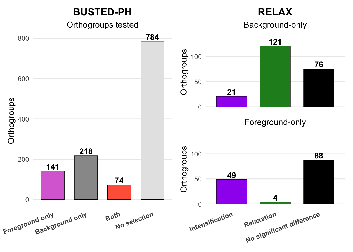
Venn diagram
# Load required packages
library(readr)
library(dplyr)
library(ggvenn)

# Load Full tree dataset
df_full <- read_csv("/Users/maevatecher/Documents/GitHub/locust-comparative-genomics/data/HYPHY_selection/ParsedRELAXResults/joint_busted_relax_annotated.csv", show_col_types = FALSE)

# Load Pruned tree dataset
df_pruned <- read_csv("/Users/maevatecher/Documents/GitHub/locust-comparative-genomics/data/HYPHY_selection/ParsedRELAXResults_Pruned/joint_busted_relax_annotated.csv", show_col_types = FALSE)

# Define helper function to get PSG + Intensification orthogroups
get_psg_intensified <- function(df) {
  df %>%
    mutate(
      k_val = as.numeric(k),
      pval = as.numeric(pval),
      selection_type = case_when(
        is.na(pval) ~ "Undetermined",
        pval < 0.05 & k_val > 1 ~ "Intensification",
        pval < 0.05 & k_val < 1 ~ "Relaxation",
        TRUE ~ "No significant difference"
      )
    ) %>%
    filter(suspect_result.x == FALSE) %>%
    filter(selection_status %in% c("Foreground only", "Both foreground and background")) %>%
    filter(selection_type == "Intensification") %>%
    pull(orthogroup) %>%
    unique()
}

# Get orthogroup sets
psg_intens_full <- get_psg_intensified(df_full)
psg_intens_pruned <- get_psg_intensified(df_pruned)

# Create named list for Venn input
venn_input <- list(
  FullTree = psg_intens_full,
  PrunedTree = psg_intens_pruned
)

# Plot Venn diagram
ggvenn(venn_input,
       fill_color = c("#66c2a5", "#fc8d62"),
       stroke_size = 0.7,
       set_name_size = 5,
       text_size = 4,
       show_percentage = FALSE) +
  ggtitle("PSGs under Intensification in swarming locusts (Full vs Pruned Tree)")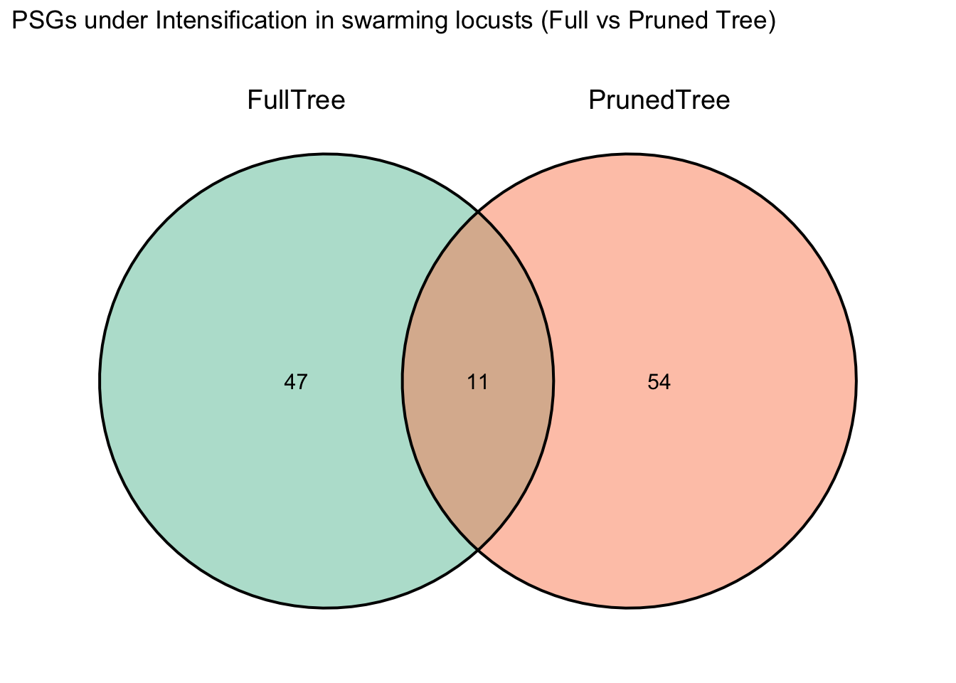
# Get the intersection of PSGs under intensification
intersect_psg_intens <- intersect(psg_intens_full, psg_intens_pruned)

# Show the result
length(intersect_psg_intens)  # Number of shared orthogroups
[1] 11intersect_psg_intens # List of orthogroup IDs [1] "OG0007006" "OG0007326" "OG0011236" "OG0011677" "OG0011869" "OG0011931"
[7] "OG0012017" "OG0012034" "OG0012129" "OG0012163" "OG0012186"For relaxation PSGs:
# Load required packages
library(readr)
library(dplyr)
library(ggvenn)

# Load Full tree dataset
df_full <- read_csv("/Users/maevatecher/Documents/GitHub/locust-comparative-genomics/data/HYPHY_selection/ParsedRELAXResults/joint_busted_relax_annotated.csv", show_col_types = FALSE)

# Load Pruned tree dataset
df_pruned <- read_csv("/Users/maevatecher/Documents/GitHub/locust-comparative-genomics/data/HYPHY_selection/ParsedRELAXResults_Pruned/joint_busted_relax_annotated.csv", show_col_types = FALSE)

# Define helper function to get PSG + Intensification orthogroups
get_psg_relaxed <- function(df) {
  df %>%
    mutate(
      k_val = as.numeric(k),
      pval = as.numeric(pval),
      selection_type = case_when(
        is.na(pval) ~ "Undetermined",
        pval < 0.05 & k_val > 1 ~ "Intensification",
        pval < 0.05 & k_val < 1 ~ "Relaxation",
        TRUE ~ "No significant difference"
      )
    ) %>%
    filter(suspect_result.x == FALSE) %>%
    filter(selection_status %in% c("Foreground only", "Both foreground and background")) %>%
    filter(selection_type == "Relaxation") %>%
    pull(orthogroup) %>%
    unique()
}

# Get orthogroup sets
psg_relax_full <- get_psg_relaxed(df_full)
psg_relax_pruned <- get_psg_relaxed(df_pruned)

# Create named list for Venn input
venn_input <- list(
  FullTree = psg_relax_full,
  PrunedTree = psg_relax_pruned
)

# Plot Venn diagram
ggvenn(venn_input,
       fill_color = c("#66c2a5", "#fc8d62"),
       stroke_size = 0.7,
       set_name_size = 5,
       text_size = 4,
       show_percentage = FALSE) +
  ggtitle("PSGs under Relaxation in swarming locusts (Full vs Pruned Tree)")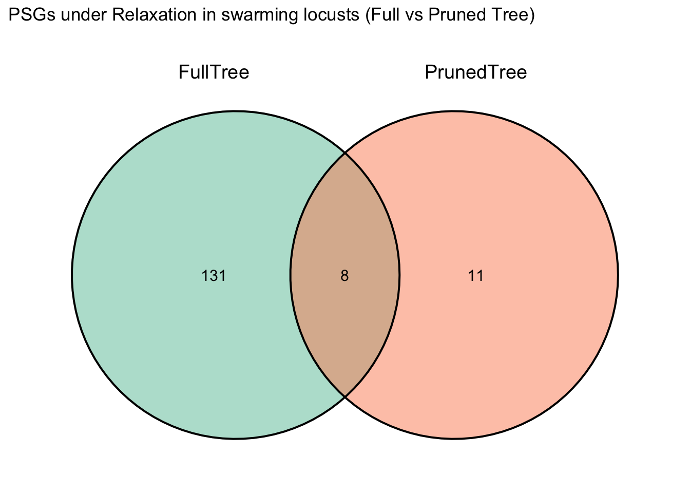
# Get the intersection of PSGs under intensification
intersect_psg_relax <- intersect(psg_relax_full, psg_relax_pruned)

# Show the result
length(intersect_psg_relax)  # Number of shared orthogroups
[1] 8intersect_psg_relax # List of orthogroup IDs[1] "OG0008483" "OG0008811" "OG0009185" "OG0011592" "OG0011838" "OG0011966"
[7] "OG0012059" "OG0012354"11. DEG and PSGs
Full tree
Here we want to know if the PSG from the BUSTED+RELAX detection share an overlap with DEGs. We extracted the list of Orthogroup DEGs (shared by the three locusts) for this step:
# Install if needed
# install.packages("VennDiagram")

library(VennDiagram)
Warning: package 'VennDiagram' was built under R version 4.4.3Loading required package: grid
Attaching package: 'grid'The following object is masked from 'package:Biostrings':
patternLoading required package: futile.loggerWarning: package 'futile.logger' was built under R version 4.4.3
Attaching package: 'VennDiagram'The following object is masked from 'package:ape':
rotatelibrary(dplyr)
library(grid)
thorax <- c(
"OG0000679", "OG0004144", "OG0000104", "OG0000015", "OG0014033", "OG0012058",
"OG0000357", "OG0000090", "OG0003126", "OG0004306", "OG0000001", "OG0009321",
"OG0015157", "OG0012103", "OG0004309", "OG0000346", "OG0000014", "OG0000796",
"OG0000151", "OG0011174", "OG0013138", "OG0000003", "OG0000391", "OG0007893",
"OG0001029", "OG0010128", "OG0001327", "OG0011184", "OG0000615", "OG0000922",
"OG0000095", "OG0012329", "OG0010429", "OG0010105", "OG0012400", "OG0012312",
"OG0000012", "OG0005229", "OG0000532", "OG0000027", "OG0000017", "OG0009757",
"OG0002737", "OG0002903", "OG0011877", "OG0003752", "OG0007957", "OG0000000",
"OG0009700", "OG0011824", "OG0000043", "OG0011853", "OG0000347", "OG0005741",
"OG0003890", "OG0000334", "OG0000419", "OG0002738", "OG0000065", "OG0000130",
"OG0000327", "OG0000093"
)
head <- c(
"OG0000104", "OG0000015", "OG0000105", "OG0004296", "OG0000371", "OG0003126",
"OG0004306", "OG0012979", "OG0009321", "OG0000073", "OG0002734", "OG0015157",
"OG0000796", "OG0000151", "OG0000222", "OG0000296", "OG0000391", "OG0000196",
"OG0010128", "OG0009808", "OG0000788", "OG0000922", "OG0000120", "OG0000212",
"OG0002726", "OG0007990", "OG0003478", "OG0000027", "OG0002737", "OG0011877",
"OG0007957", "OG0009113", "OG0000334", "OG0000823", "OG0002738", "OG0000093",
"OG0000552", "OG0000553"
)
all_degs <- unique(c(thorax, head))
# Load Pruned tree dataset
df_pruned <- read_csv("/Users/maevatecher/Documents/GitHub/locust-comparative-genomics/data/HYPHY_selection/ParsedRELAXResults/joint_busted_relax_annotated.csv", show_col_types = FALSE)
# Recalculate selection_type from k and pval
df <- df_pruned %>%
mutate(
k_val = as.numeric(k),
pval = as.numeric(pval),
padj = as.numeric(padj),
selection_type = case_when(
is.na(pval) ~ "Undetermined",
pval < 0.05 & k_val > 1 ~ "Intensification",
pval < 0.05 & k_val < 1 ~ "Relaxation",
TRUE ~ "No significant difference"
)
)
# Filter non-suspect orthogroups
df_suspect <- df %>%
filter(selection_status != "No selection") %>%
filter(suspect_result.x == FALSE) %>%
mutate(
PSG = selection_status %in% c("Foreground only", "Both foreground and background"),
Relaxation = selection_type == "Relaxation",
Intensification = selection_type == "Intensification",
Insignificant = selection_type == "No significant difference"
) %>%
dplyr::select(orthogroup, PSG, Relaxation, Intensification, Insignificant) %>%
distinct()
# Add color groups: PSG > Relaxation > Other
df_suspect <- df_suspect %>%
mutate(
PSG_color = case_when(
PSG ~ "PSG",
Relaxation ~ "Relaxation",
Intensification ~ "Intensification",
TRUE ~ "Other"
)
)
# Define color palette
custom_colors <- c(
"PSG" = "orchid", # Green
"Relaxation" = "gold", # Orange
"Intensification" = "tomato", # Orange
"Other" = "black" # Default gray
)
# Reorder factor levels BEFORE calling upset()
df_suspect_long <- df_suspect %>%
pivot_longer(cols = c("PSG", "Relaxation", "Intensification", "Insignificant"),
names_to = "set", values_to = "value") %>%
filter(value) %>%
mutate(set = factor(set, levels = c("Insignificant", "Intensification", "Relaxation", "PSG"))) %>%
pivot_wider(names_from = set, values_from = value, values_fill = FALSE)
# Add color groups again
df_suspect_long <- df_suspect_long %>%
mutate(
PSG_color = case_when(
PSG ~ "PSG",
Relaxation ~ "Relaxation",
Intensification ~ "Intensification",
TRUE ~ "Other"
)
)
# Extract PSGs from your annotated dataframe
psgs <- df_suspect_long %>%
filter(PSG) %>%
pull(orthogroup) %>%
unique()
# Draw the Venn diagram
venn.plot <- draw.pairwise.venn(
area1 = length(psgs),
area2 = length(all_degs),
cross.area = length(intersect(psgs, all_degs)),
category = c("PSGs", "DEGs"),
fill = c("orchid", "deepskyblue"),
lty = "blank",
cex = 2,
cat.cex = 2,
cat.pos = c(-20, 20),
cat.dist = c(0.05, 0.05)
)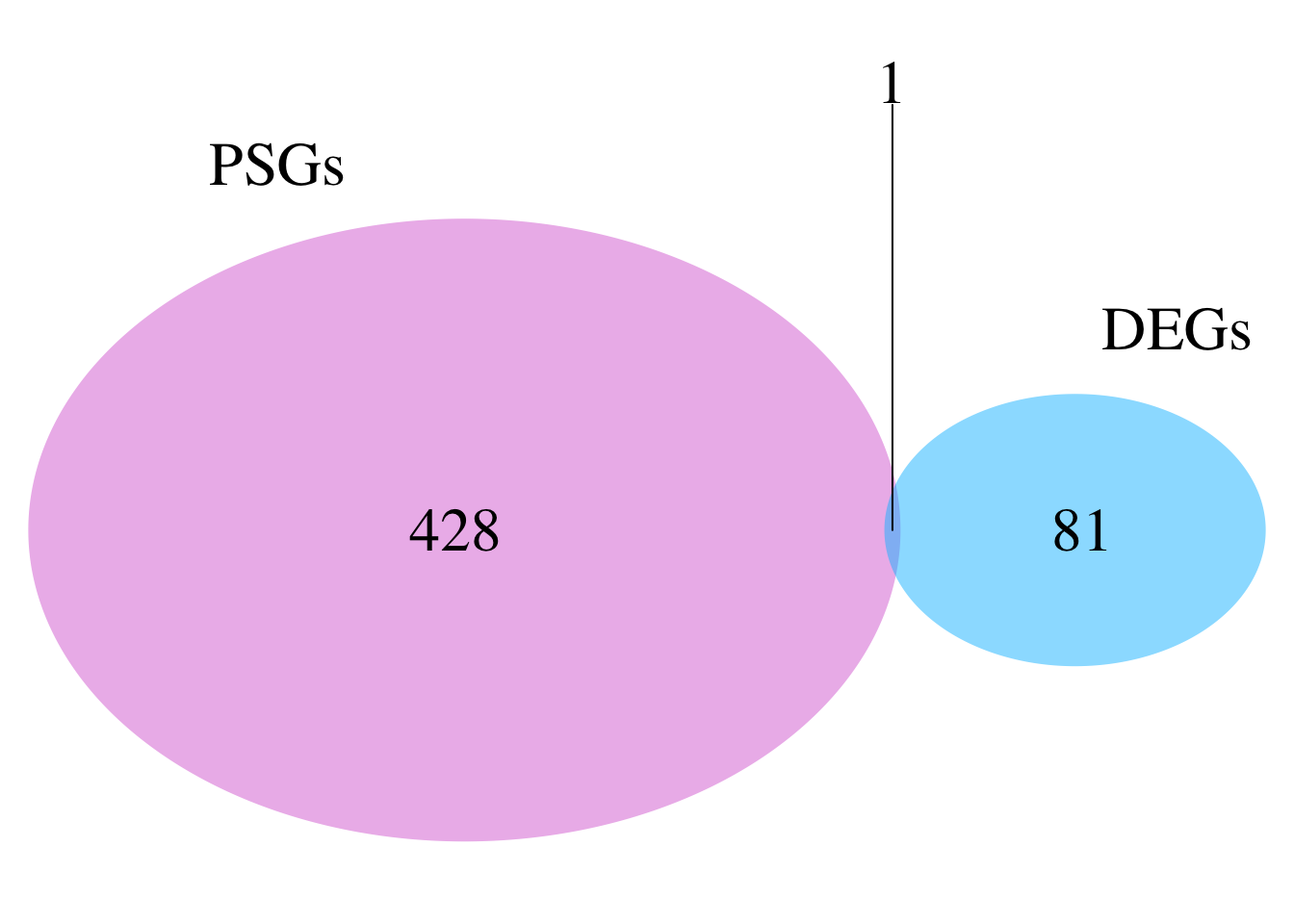
# Display the plot
grid.newpage()
grid.draw(venn.plot)
# Get the intersection of PSGs under intensification
intersect_psg_deg <- intersect(psgs, all_degs)

# Show the result
length(intersect_psg_deg)  # Number of shared orthogroups
[1] 1intersect_psg_deg # List of orthogroup IDs[1] "OG0012312"Pruned tree
Here we want to know if the PSG from the BUSTED+RELAX detection share an overlap with DEGs. We extracted the list of Orthogroup DEGs (shared by the three locusts) for this step:
# Install if needed
# install.packages("VennDiagram")

library(VennDiagram)
library(dplyr)
library(grid)

thorax <- c(
  "OG0000679", "OG0004144", "OG0000104", "OG0000015", "OG0014033", "OG0012058",
  "OG0000357", "OG0000090", "OG0003126", "OG0004306", "OG0000001", "OG0009321",
  "OG0015157", "OG0012103", "OG0004309", "OG0000346", "OG0000014", "OG0000796",
  "OG0000151", "OG0011174", "OG0013138", "OG0000003", "OG0000391", "OG0007893",
  "OG0001029", "OG0010128", "OG0001327", "OG0011184", "OG0000615", "OG0000922",
  "OG0000095", "OG0012329", "OG0010429", "OG0010105", "OG0012400", "OG0012312",
  "OG0000012", "OG0005229", "OG0000532", "OG0000027", "OG0000017", "OG0009757",
  "OG0002737", "OG0002903", "OG0011877", "OG0003752", "OG0007957", "OG0000000",
  "OG0009700", "OG0011824", "OG0000043", "OG0011853", "OG0000347", "OG0005741",
  "OG0003890", "OG0000334", "OG0000419", "OG0002738", "OG0000065", "OG0000130",
  "OG0000327", "OG0000093"
)

head <- c(
  "OG0000104", "OG0000015", "OG0000105", "OG0004296", "OG0000371", "OG0003126",
  "OG0004306", "OG0012979", "OG0009321", "OG0000073", "OG0002734", "OG0015157",
  "OG0000796", "OG0000151", "OG0000222", "OG0000296", "OG0000391", "OG0000196",
  "OG0010128", "OG0009808", "OG0000788", "OG0000922", "OG0000120", "OG0000212",
  "OG0002726", "OG0007990", "OG0003478", "OG0000027", "OG0002737", "OG0011877",
  "OG0007957", "OG0009113", "OG0000334", "OG0000823", "OG0002738", "OG0000093",
  "OG0000552", "OG0000553"
)

all_degs <- unique(c(thorax, head))

# Load Pruned tree dataset
df_pruned <- read_csv("/Users/maevatecher/Documents/GitHub/locust-comparative-genomics/data/HYPHY_selection/ParsedRELAXResults_Pruned/joint_busted_relax_annotated.csv", show_col_types = FALSE)


# Recalculate selection_type from k and pval
df <- df_pruned %>%
  mutate(
    k_val = as.numeric(k),
    pval = as.numeric(pval),
    padj = as.numeric(padj),
    selection_type = case_when(
      is.na(pval) ~ "Undetermined",
      pval < 0.05 & k_val > 1 ~ "Intensification",
      pval < 0.05 & k_val < 1 ~ "Relaxation",
      TRUE ~ "No significant difference"
    )
  )

# Filter non-suspect orthogroups
df_suspect <- df %>%
  filter(selection_status != "No selection") %>%
  filter(suspect_result.x == FALSE) %>%
  mutate(
    PSG = selection_status %in% c("Foreground only", "Both foreground and background"),
    Relaxation = selection_type == "Relaxation",
    Intensification = selection_type == "Intensification",
    Insignificant = selection_type == "No significant difference"
  ) %>%
  dplyr::select(orthogroup, PSG, Relaxation, Intensification, Insignificant) %>%
  distinct()

# Add color groups: PSG > Relaxation > Other
df_suspect <- df_suspect %>%
  mutate(
    PSG_color = case_when(
      PSG ~ "PSG",
      Relaxation ~ "Relaxation",
      Intensification ~ "Intensification",
      TRUE ~ "Other"
    )
  )

# Define color palette
custom_colors <- c(
  "PSG" = "orchid",         # Green
  "Relaxation" = "gold",   # Orange
  "Intensification" = "tomato",   # Orange
  "Other" = "black"         # Default gray
)


# Reorder factor levels BEFORE calling upset()
df_suspect_long <- df_suspect %>%
  pivot_longer(cols = c("PSG", "Relaxation", "Intensification", "Insignificant"),
               names_to = "set", values_to = "value") %>%
  filter(value) %>%
  mutate(set = factor(set, levels = c("Insignificant",  "Intensification", "Relaxation", "PSG"))) %>%
  pivot_wider(names_from = set, values_from = value, values_fill = FALSE)

# Add color groups again
df_suspect_long <- df_suspect_long %>%
  mutate(
    PSG_color = case_when(
      PSG ~ "PSG",
      Relaxation ~ "Relaxation",
      Intensification ~ "Intensification",
      TRUE ~ "Other"
    )
  )


# Extract PSGs from your annotated dataframe
psgs <- df_suspect_long %>%
  filter(PSG) %>%
  pull(orthogroup) %>%
  unique()


# Draw the Venn diagram
venn.plot <- draw.pairwise.venn(
  area1 = length(psgs),
  area2 = length(all_degs),
  cross.area = length(intersect(psgs, all_degs)),
  category = c("PSGs", "DEGs"),
  fill = c("orchid", "deepskyblue"),
  lty = "blank",
  cex = 4,
  cat.cex = 2,
  cat.pos = c(-20, 20),
  cat.dist = c(0.05, 0.05)
)
# Display the plot
grid.newpage()
grid.draw(venn.plot)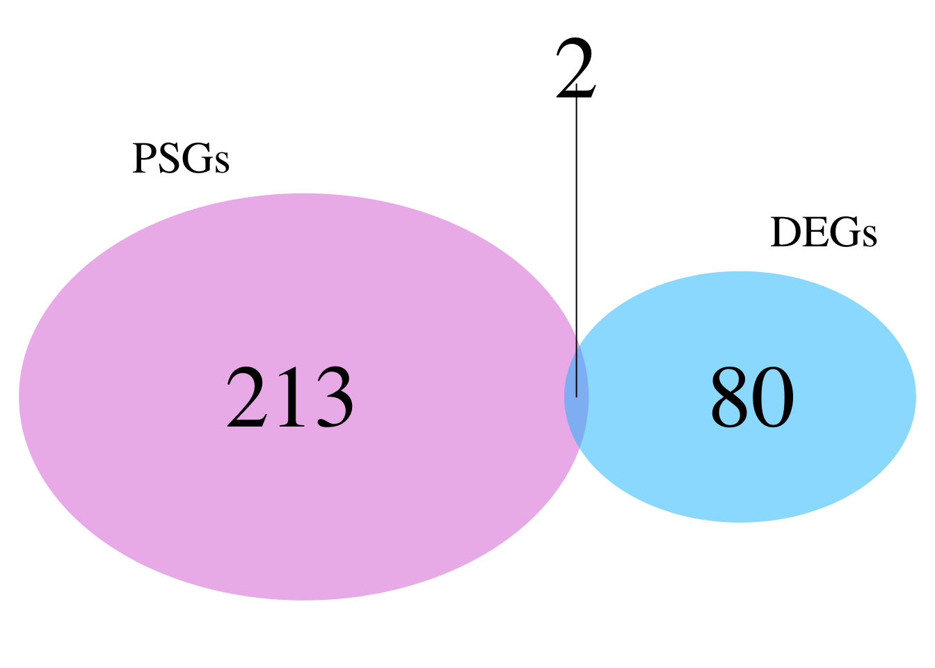
# Get the intersection of PSGs under intensification
intersect_psg_deg <- intersect(psgs, all_degs)

# Show the result
length(intersect_psg_deg)  # Number of shared orthogroups
[1] 2intersect_psg_deg # List of orthogroup IDs[1] "OG0010128" "OG0012312"
sessionInfo()R version 4.4.2 (2024-10-31)
Platform: aarch64-apple-darwin20
Running under: macOS Sequoia 15.7.4
Matrix products: default
BLAS: /Library/Frameworks/R.framework/Versions/4.4-arm64/Resources/lib/libRblas.0.dylib
LAPACK: /Library/Frameworks/R.framework/Versions/4.4-arm64/Resources/lib/libRlapack.dylib; LAPACK version 3.12.0
locale:
[1] en_US.UTF-8/en_US.UTF-8/en_US.UTF-8/C/en_US.UTF-8/en_US.UTF-8
time zone: Asia/Tokyo
tzcode source: internal
attached base packages:
[1] grid stats4 stats graphics grDevices utils datasets
[8] methods base
other attached packages:
[1] VennDiagram_1.8.2 futile.logger_1.4.9 ggvenn_0.1.19
[4] patchwork_1.3.2 ComplexUpset_1.3.6 plotly_4.11.0
[7] ggnewscale_0.5.2 kableExtra_1.4.0 knitr_1.51
[10] DesertLocustR_0.1.0 remotes_2.5.0 Biostrings_2.74.1
[13] XVector_0.46.0 AnnotationHub_3.14.0 BiocFileCache_2.14.0
[16] dbplyr_2.5.1 rtracklayer_1.66.0 GenomicRanges_1.58.0
[19] GenomeInfoDb_1.42.3 GO.db_3.20.0 AnnotationDbi_1.68.0
[22] IRanges_2.40.1 S4Vectors_0.44.0 Biobase_2.66.0
[25] BiocGenerics_0.52.0 clusterProfiler_4.14.6 data.table_1.18.0
[28] lubridate_1.9.4 forcats_1.0.1 stringr_1.6.0
[31] purrr_1.2.1 tibble_3.3.1 tidyverse_2.0.0
[34] viridis_0.6.5 viridisLite_0.4.2 ape_5.8-1
[37] ggVennDiagram_1.5.7 multcompView_0.1-10 tidyr_1.3.2
[40] broom_1.0.12 readr_2.1.6 dplyr_1.1.4
[43] ggplot2_4.0.2 workflowr_1.7.2
loaded via a namespace (and not attached):
[1] splines_4.4.2 later_1.4.5
[3] BiocIO_1.16.0 bitops_1.0-9
[5] ggplotify_0.1.3 filelock_1.0.3
[7] R.oo_1.27.1 XML_3.99-0.20
[9] lifecycle_1.0.5 rprojroot_2.1.1
[11] processx_3.8.6 lattice_0.22-7
[13] vroom_1.6.7 crosstalk_1.2.2
[15] backports_1.5.0 magrittr_2.0.4
[17] sass_0.4.10 rmarkdown_2.30
[19] jquerylib_0.1.4 yaml_2.3.12
[21] httpuv_1.6.16 otel_0.2.0
[23] ggtangle_0.1.1 cowplot_1.2.0
[25] DBI_1.2.3 RColorBrewer_1.1-3
[27] abind_1.4-8 zlibbioc_1.52.0
[29] R.utils_2.13.0 RCurl_1.98-1.17
[31] yulab.utils_0.2.3 rappdirs_0.3.4
[33] git2r_0.36.2 GenomeInfoDbData_1.2.13
[35] enrichplot_1.26.6 ggrepel_0.9.6
[37] tidytree_0.4.7 svglite_2.2.2
[39] codetools_0.2-20 DelayedArray_0.32.0
[41] xml2_1.5.2 DOSE_4.0.1
[43] tidyselect_1.2.1 aplot_0.2.9
[45] UCSC.utils_1.2.0 farver_2.1.2
[47] matrixStats_1.5.0 GenomicAlignments_1.42.0
[49] jsonlite_2.0.0 systemfonts_1.3.1
[51] tools_4.4.2 ragg_1.5.0
[53] treeio_1.30.0 Rcpp_1.1.1
[55] glue_1.8.0 gridExtra_2.3
[57] SparseArray_1.6.2 xfun_0.56
[59] qvalue_2.38.0 MatrixGenerics_1.18.1
[61] withr_3.0.2 formatR_1.14
[63] BiocManager_1.30.27 fastmap_1.2.0
[65] callr_3.7.6 digest_0.6.39
[67] timechange_0.3.0 R6_2.6.1
[69] gridGraphics_0.5-1 textshaping_1.0.4
[71] colorspace_2.1-2 dichromat_2.0-0.1
[73] RSQLite_2.4.5 R.methodsS3_1.8.2
[75] hexbin_1.28.5 utf8_1.2.6
[77] generics_0.1.4 htmlwidgets_1.6.4
[79] httr_1.4.7 S4Arrays_1.6.0
[81] whisker_0.4.1 pkgconfig_2.0.3
[83] gtable_0.3.6 blob_1.3.0
[85] S7_0.2.1 htmltools_0.5.9
[87] fgsea_1.32.4 scales_1.4.0
[89] png_0.1-8 ggfun_0.2.0
[91] lambda.r_1.2.4 rstudioapi_0.18.0
[93] tzdb_0.5.0 reshape2_1.4.5
[95] rjson_0.2.23 nlme_3.1-168
[97] curl_7.0.0 cachem_1.1.0
[99] BiocVersion_3.20.0 parallel_4.4.2
[101] restfulr_0.0.16 pillar_1.11.1
[103] vctrs_0.7.0 promises_1.5.0
[105] evaluate_1.0.5 futile.options_1.0.1
[107] cli_3.6.5 compiler_4.4.2
[109] Rsamtools_2.22.0 rlang_1.1.7
[111] crayon_1.5.3 labeling_0.4.3
[113] ps_1.9.1 getPass_0.2-4
[115] plyr_1.8.9 fs_1.6.6
[117] stringi_1.8.7 BiocParallel_1.40.2
[119] lazyeval_0.2.2 GOSemSim_2.32.0
[121] Matrix_1.7-4 hms_1.1.4
[123] bit64_4.6.0-1 KEGGREST_1.46.0
[125] SummarizedExperiment_1.36.0 igraph_2.2.1
[127] memoise_2.0.1 bslib_0.9.0
[129] ggtree_3.14.0 fastmatch_1.1-8
[131] bit_4.6.0 gson_0.1.0